Offline Reinforcement Learning

Tags	CS 224RCS 285Reviewed 2024

Further reading

The setting

Suppose that you had an environment and you have a bunch of trajectories in the environment. Can you run RL on it? This is known as offline RL.

In this first section, we will be focusing on policy evaluation; given data about the environment, can we see how good a new policy will do?

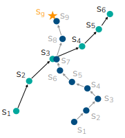
Why is this hard? Well, in normal RL, you can try things as needed. In offline RL, what you don’t know will stay that way. But it is worth mentioning that unlike imitation learning, you have an opportunity to stitch trajectories together to find a better one.

Why not just imitation learn?

Well, imitation learning will only follow expert actions. There is no notion (in vanilla BC) of which is better and worse. In contrast, offline RL can stitch together trajectories

However, it’s worth mentioning that offline RL can’t just find a perfect path if there doesn’t exist one. Even if it’s obvious, a good offline RL algorithm can’t stray far from the existing data out of fear of OOD problems. So we just need to have some degree of goodness in the data.

Why Offline RL?

In the real world, it’s not optimal to do trial and error in real life. Rather, it’s better to tap into a dataset and then finetune in real life (or even zero-shot work in real life). The key benefit is that we can reuse datasets, just like imagenet!

Unfortunately, there is still a pretty big gap that we need to cross before this becomes a reality.

Common assumptions

stationary process: the environment will be the same as the dataset

Sequential ignorability: all the data relevant for control is included in the state

Overlap: the data collection policy should explore a space larger than the policy you wish to evaluate (if this is not done, then the estimate can’t be correct)

Evaluation criteria

efficiency in computation

performance accuracy: compare the yielded $\hat{V}^\pi$ to the true $V^\pi$
- MSE between value functions
- Limit behavior: is the estimation unbiased, i.e. as the data goes to infinity, do we yield the true $V\pi$ ?
- Boundable: is it possible to say that the estimate is within a certain range of the true value, as a function of the dataset size?

Malignant distribution shift

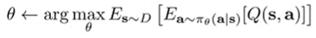
The classical setup is ERM (formulated in a distribution)

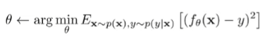
If you have a new set $\bar x$ , it’s generally true that the $\theta$ found under $p(x)$ is the same $\theta$ found under your $p(\bar x)$ . Usually, neural networks generalize pretty well. So generalization isn’t the exact problem of why naively applying RL to offline datasets doesn’t work.

The problem arises because the $x$ isn’t picked randomly; it’s picked adversarially to maximize the existing Q function. Any false optimism is rewarded and propagated through the MSE objective during the training of the Q function

Evaluating the behavior policy

If we just want to evaluate the behavior policy, we can run some existing algorithm, because the problem of malignant distribution shift doesn’t exist.

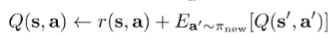
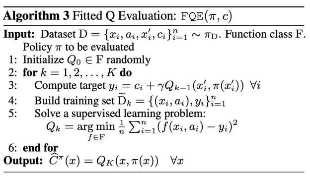
We use the fitted Q evaluation algorithm, which is very similar to DQN, except that we don’t run any argmax over Q to get a policy (because in this case, we have a policy already).

Algorithm

There are some theoretical guarntees we can make on the distance between the approximated and the real value function through a PAC condition:

Bound
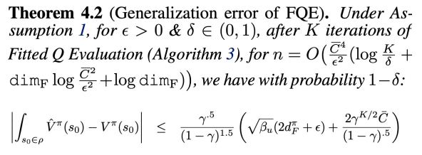
where $dim_F$ si the size of your policy class $F$ and $C$ is related to the overlap between the sampling policy and the evaluation policy. The less you overlap, the more samples you need.
We also define $d^\pi_F$ as
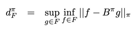
which intuitively means, given some arbitrary function $g$ , you do a bellman backup, and then you try to fit a function $f$ to it (essentailly run one round of the fitted Q evaluation algorithm), how large can this error be? In other words, suppose you run the fitted Q eval algorithm. What is the largest loss that can be incurred during the fitting stage? We compute the loss by weighting an L2 norm WRT policy.
This bound essentially gives you a PAC bound for the distance between value functions. From it, you can derive how many samples you’d need to use. This bound is true for any function class.

Evaluation using Importance Sampling

Let’s say we wanted to evaluate some policy using data from a different behavior policy. One idea is to use importance sampling

Note that under this setup, we need access to the density of the behavior policy, which can be challenging. Let’s get back to this problem later.

The exponential cost

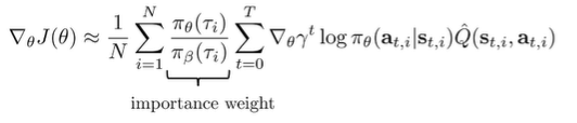
In policy gradient, we realized that the importance samples were pretty nasty, so we used workarounds. However, we can’t use these workarounds because our policies can actually be quite different.

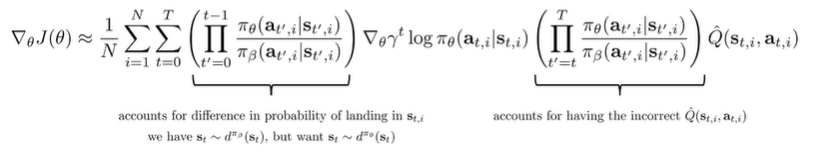
Note that our cost is still exponential in $T$ , which is not good. We can use commutative property to split up the products between the log term and the Q term, and we can potentially ignore the first products from $0→t$ . We can assume that the state distributions are similar. However, the second product from $t→T$ can’t be ignored.

The unfortunate reality is that this exponential problem will pervade, no matter what you do. But there are some methods that reduce the problem a little bit

Doubly Robust Estimator

💡

See: Doubly Robust off-policy value evaluation for reinforcement learning

Let’s focus on estimating the value function of the policy, which can be very helpful.

💡

Note that we are just using

s_0

for notational simplicity.

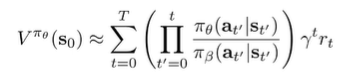
If we let $\rho_t = \pi_\theta / \pi_\beta$ , we can write this summation-product out completely

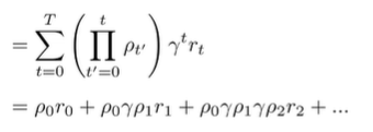
Which we set equal to $\bar{V}^T$ as the estimator to $V^{\pi_0}(s_0)$ . You can create this $\bar{V}^T$ using a nice recursive structure which should be apparent in the rollout above

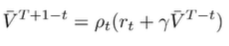
And this gives us a bellman-like update for creating a value function estimate. To complete this Doubly Robust estimator, we add a baseline modification by adding $\hat{V}$ and subtracting $\hat{Q}$ . We won’t go into too much details, but essentially you’re just creating a modified way of fitting $\bar{V}^T$ , which approximates the true value function.

Marginalized Importance Sampling

Can we estimate

w(s, a) = \frac{d^{\pi_\theta}(s,a)}{d^{\pi_\beta}(s,a)}

💡

Recall:

d(s, a)

is the marginal state-action density.

which doesn’t suffer from the exponential problem. If we had this, then we can estimate $J(\theta) = E_{d^{\pi_\beta}}[w(s, a)r]$ , where the expectation is taken Monte Carlo from the dataset. If you write out the summation of this expectation, you’ll see that it is exactly the RL objective. But how do we determine $w$ ?

One method is to enforce a certain equality (Zhang et al., GenDICE)

And this is just a truism about the the marginal state-action density if you write out the definition of $w$ . We won’t go into too much detail here, but this is just one idea.

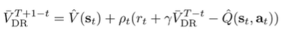
Additional reading

Offline RL using Linear Fitted Value Functions

If we assume very simple functions and ditch the problem of maximization bias, we can derive a closed-form solution that solves for the value function using offlien data.

Model-based Value Estimation

Let’s say that we have a feature matrix $\Phi$ which is $|S| \times K$ , meaning that every state has some feature representation. Let’s assume that the reward is $\Phi w_r \approx r$ . The least squares solution is $w_r = (\Phi^T\Phi)^{-1}\Phi^Tr$ if we are given $r$ , which is the reward for all state-action tuples.

To create a transition, just compute $P^\pi \Phi$ . Of course, this is policy specific because a policy takes in a state and decides what to do. Now, this is the ideal, but it may not be tractable. Instead, you want to find a matrix $P_\Phi$ such that

\Phi P_{\Phi} \approx P^\pi \Phi

Essentially, you’re embedding your transitions into feature space! Just like the reward model, it’s $P_\Phi = (\Phi^T\Phi)^{-1}P^\pi\Phi$

With all of these, we can try estimating the value function using $\Phi w_V$ . To do this, we note that the bellman equation is $V^\pi = r + \gamma P^\pi V^\pi$ . And we can solve for the value function

V^\pi = (I -\gamma P^\pi)^{-1}r

And you can do the same thing in feature space

w_V = (I - \gamma P_\Phi)^{-1}w_r

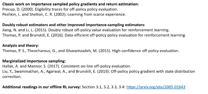
Now, let’s substitute in our world definitions into the feature space.

and this is called the least-squares temporal difference (LSTD). This is a very powerful formulation, because it allows you to compute the parameters to $V^\pi$ using knowledge about the world.

This is a powerful method, but can we also get desirable results by using samples instead of world models?

Working with samples

If we can replace the model with samples, this approach now becomes model-free. Let’s let $\Phi$ be a $|D|\times K$ matrix, and replace $P^\pi \Phi%$ with $\Phi’$ , which are the features at the next time step (we can get the next step from the $s, a, s’$ in the dataset. We also replace $r$ with a $|D|$ vector, instead of a $|S|$ vector.

And interestingly, the equation we derived above will work the same way with the sample approximation

w_v = (\Phi^T\Phi - \gamma \Phi^T \Phi')^{-1}\Phi^Tr

The unfortunate barrier is that $\Phi’$ is policy-specific which means that we can use this equation to estimate the policy that collected the data (i.e. $\pi_\beta$ ), but NOT any other policy, which we might be learning from the offline data.

As a quick solution, we can replace Value function estimation with Q function estimation, which decouples it from the policy. To do this, we define $\Phi \in |S||A| \times K’$ . Everything else stays exactly the same. For the $\Phi’$ , we choose the action that the policy would have taken in this next step (sort of like a regular bellman backup).

Problem with linear approach

The issue is that the linear approach will use the same bellman backup equation

because it’s using least squares. The adversarial maximization bias still exists.

Policy constraint methods

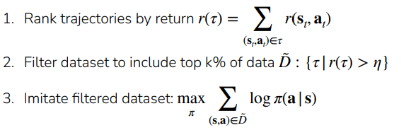
Zeroth try: Filtered Behavior Cloning 💻

The algorithm is simple: select the trajectories from the demonstrations with a large enough reward, and then run BC on it. This prevents lower performance trajectories from being used.

Algorithm

First try: explicit policy constraints

As inspired from policy gradients, we can try to set up a trust region around our behavior policy such that our optimized $\pi$ and the behavior policy $\pi_\beta$ are close, using some sort of metric like DKL:

D_{KL}(\pi_\theta || \pi_\beta) < \epsilon

Unfortunately, there are two big problems:

We don’t know the $\pi_\beta$ , which means that we either fit another model with BC, or we need to be clever to implement the constraint, such that we use samples and not probability densities

This is often too pessimistic (you want to do better than $\pi_\beta$ , which requires you to be different. But at the same time, this blanket constraint may not be pessimistic enough when pessimism matters more. So you can get the worst of both worlds.

Additional reading

We can also try a support constraint, i.e. you set $\pi(a | s) \geq 0$ only if $\pi_\beta(a |s)\geq \epsilon$ . Unfortuatnely, this is hard to implement, although this is closer to what we want.

Implementing explicit policy constraint methods

You can just modify the actor objective. If you use KL divergence, you can write this as following:

Remember that the actor objective is the following

So because they are under the same expectation, we can just smush them together

The $\lambda$ comes from constrained optimization. We can use dual gradient descent to find $\lambda$ , or we can treat it as a hyperparameter. In general, this modified objective is easy to compute, except that you don’t know $\pi_\beta$ . So, you might train another policy that approximates $\pi_\beta$ , but this can be a hassle.

Instead, we can consider modifying the reward function to penalize KL divergence.

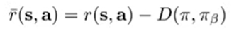
This actually also avoids future divergence, which can be quite desirable (it’s got a larger window)

Implicit Policy Constraint (AWR, AWAC)

If we solve this constraint equation,

we get the closed form solution

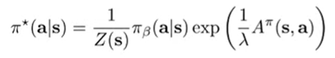
So here’s the intuition. It’s making suboptimal actions exponentially less likely, but we also consider the likelihood of this action under the behavior policy.

Of course, we can’t do this because we need to know $\pi_\beta$ . However, we do have access to samples from $\pi_\beta$ , which means that we can turn the optimal formula into an objective:

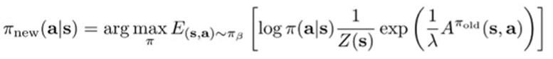
This is basically the behavior cloning loss with an advantage weight, hence why this is called advantage weighted regression. In AWR, the advantage is estimated in a Monte Carlo way.

To reduce variance, we can use an actor-critic approach where we learn a Q function. This is known as Advantage Weighted Actor Critic, or AWAC:

Algorithm

☝

This is VERY similar to policy gradient, which maximizes

E[\pi(a|s) A(s,a)]

. One key difference is the source of data. Policy gradient uses online data, while weighted BC uses offline data.

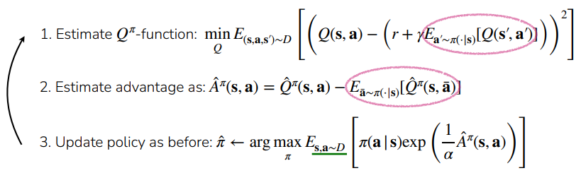
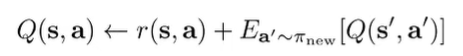
The only problem is that we may be querying OOD actions in the Q function in two places: first, when we compute the $\mathcal{L}_C$ inner expectation. The second place is when we are estimating $A = Q - E_{\pi_\theta} Q$ . Can we avoid this all together?

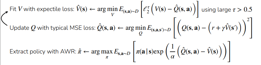
Avoiding OOD in Q update (Implicit Q Learning, IQL)

AWAC was good, but we want to continue eliminate overestimation problem. We could try replacing the expectation with a value function $V(s’)$ . But how would we fit this value function? We can’t just use samples from $\pi_\beta(a|s)$ because we want the value function of $\pi_{new}$

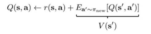
What if we can take a more optimistic expectation over $\pi_\beta$ ? For example, what if we took the expectation of the upper $n$ th percentile of $Q(s, a)$ over data induced by $\pi_\beta$ ?

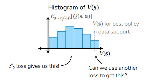
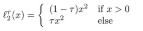
To do this, we use the target $y = E_{a’ \sim \pi_\beta}[Q(s’, a’)]$ , but instead of symmetric MSE, we use an Expectile Loss, which can be tuned to penalize negative errors more than positive errors (so we try to think of better policies than the behavior policy)

And this is better than blind maximization because everything you’re fitting is in distribution. Formally, we are training the following objective:

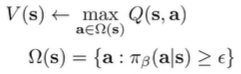
Which states that we are maximizing across seen states. This objective allows stitching because it’s on the state-level.

This approach is known as Implicit Q learning. The key insight here is that we always query $Q$ inside its support, which means that we eliminate the overestimation problem altogether.

Algorithm

Conservative Q learning (CQL)

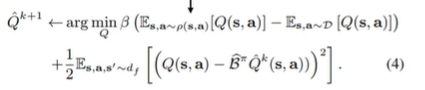
The Conservative Q Learning approach is simple: using a maximization distribution $\mu$ (more on this in a sec), let’s push down the highest Q that are not in the dataset distribution.

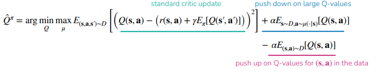
Now, this objective is nuanced. Note how if we stumble upon something in $D$ and $\mu$ , then the blue and pink components cancel. Only when $\mu$ finds something out of $D$ when the two components don’t cancel, yielding a non-zero loss that pushes down the selected Q value. In effect, this objective actively seeks and smoothes OOD overestimation.

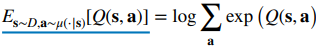
But how do we find $\mu$ ? So this isn’t completely trivial, but we can use a neat trick of math. If we assume that we add an entropy regularizer to the loss function $R(\mu) = H(\mu | S)$ , then the optimal maximizer $\mu$ becomes $\mu(a|s) \propto \exp(Q(s,a))$ . Therefore, you can use this as follows:

If we don’t use the pink term in the CQL, then we can show that the regularized $\hat{Q} < Q$ for all $s, a$ . With the pink term, we lose the element-wise guarantees, but we can still guarantee that

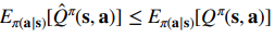
for all $s\in D$ . This is pretty good, as we are saying that the average action value is less than reality, meaning that there isn’t too much overestimation.

As an intuition: if we let $\mu$ be the softened Q function, we’re just basically trying to sharpen up a policy if it uses resources inside the dataset. Otherwise, it smoothes it out.

Comparing and contrasting

policy constraints are intuitive but often too conservative

conservative Q learning approaches are simple and work well, but require the $\alpha$ to be tuned correctly.

Offline Model-based RL

The setting is this: you’re given an experience dataset. How can you learn a good model-based policy? If we are not careful, our policy optimization might exploit flaws in the dynamics model. It’s just like Q learning: without environment feedback, we have the problem of over-optimism

MOPO (model based offline policy optimization)

This is just DYNA + penalties. The idea is basically punish the policy for exploiting the model by assigning a reward function penalty for going to states where the model might be uncertain

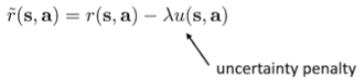
if we pick the right $\lambda$ , we punish the model more for “cheating” than it gains. But how do we quantify uncertainty? Well, one idea is using an ensemble method, where you take the standard deviation of the ensemble as a measurement of uncertainty.

COMBO (conservative model-based RL)

Basically like CQL + DYNA. The only difference is that we are pushing state and actions from the model (instead of just the actions from the learned policy)

We minimize Q values over state-action tuples provided by the model, but we concurrently maximize Q values provided by the behavior dataset. This encourages the model to stay within the behavior support. This also means that we set up a little pressure for the model to produce things that are indistinguishable from the behavior policy, because then the two terms would cancel out.

Transformer Methods

Conditional Imitation

So there also exists a much simpler solution, which is to condition the policy on the empirical reward-to-go. The objective is as follows:

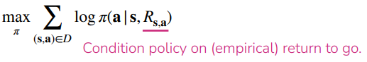
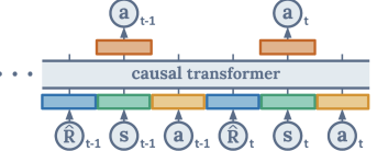
And during test-time, you just provide a very high reward and hope the model tries the hardest. Of course, there are a ton of potential problems with this setup. You can’t just put a very high number into the reward; it may be out of distribution. We can also use a causal transformer (Decision Transformer) that takes in rewards, states, and actions, and outputs optimal actions.

Trajectory Transformer

💡

See: Reinforcement learning as one big sequence modeling problem

You can train a joint state-action model, and optimize for a sequence of states and actions (instead of a single transition). With the sequence, we are able to use an expressive model like a transformer.

This transformer’s tokens are each dimension of the states and actions, discretized. It seems a little weird, and perhaps it is. But it does work!

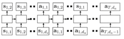
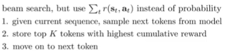
You can actually make very accurate predictions for many steps in the future. This means that you can use this model to do planning. You can use a beam search, which looks something like

What should I use?

If you train only offline, use CQL. You can also use IQL, but it has more hyperparameters.

If you train offline and finetune online, use AWAC. CQL is too conservative to fine-tune. IQL is also pretty good, and can outperform AWAC. All of these methods are easily adaptable to online training (nothing changes)

If you have a good way of training models, then COMBO is a good choice. It’s basically CQL but with models. Trajectory transformer is also good, but it’s compute-expensive.