What do we want?

Previously, we talked about policy evaluation. We had

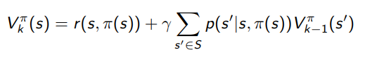
While this is valid, the problem is that we assume access to the environment transition distribution. This is actually a pretty strong assumption. So if we remove this assumption, how do we get our value function?

Monte Carlo Methods

Here’s first big idea: we know that the value function is actually the expectation over trajectories, if we write it out in non-dynamic programing form

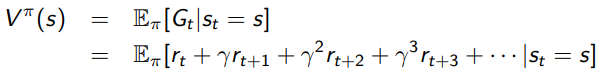
Monte Carlo approaches is all about approximating an expectation through samples. So…can we somehow average rollouts to get the value for each state?

For notation, let $G_{i, t}$ be the rollout return of trajectory $i$ in time step $t$.

First Visit / Every Visit Monte Carlo 💻

The idea of a first-visit Monte Carlo is the following

1. Initialize $N(s) = 0, G(s) = 0$. N will be a state counter, and G will be a cumulative return counter.

2. look through a trajectory. The first time a state $s$ is visited in a trajectory…
   1. $N(s) \leftarrow N(s) + 1$
   2. $G(s) \leftarrow G(s) + G_{i, t}$
   3. $V^\pi(s) \leftarrow G(s)/N(s)$

This is a really intuitive thing. You basically average the discounted return across the episodes that it shows up. We call it first visit because you only sum the first time you see a state in a rollout.

For an every visit Monte Carlo, you do the exact same thing except you ignore the “first time” qualifier. Every time you see a state $s$, you do the estimate update.

Incremental Monte Carlo 💻

Here is a slightly different way of doing things. It might seem a bit weird at first, but we’ll get to why we care about this method. In fact (spoiler alert) this is the same as every-state Monte Carlo

1. Initialize $N(s) = 0, G(s) = 0$. N will be a state counter, and G will be a cumulative return counter.

2. For every state $s$ visited…
   1. $N(s) \leftarrow N(s) + 1$
   2. $V^\pi(s) \leftarrow V^\pi(s) \frac{N(s) - 1}{N(s)} + \frac{G_{i, t}}{N(s)}$

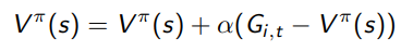
Intuitively, you can interpret the assignment as a weighted averaging between the old and the new. We can also rewrite it as

So this should make your spidey-senses tingle a bit. It looks like the second part is an “error signal” and you’re moving the value function to compensate. This actually makes sense, because $G_{i, t}$ is exactly what $V^\pi(s)$ is trying to estimate! (think about this for a second)

Properties of Incremental Monte Carlo

Let’s consider the more general incremental Monte Carlo update

We see some neat properties with different value of $\alpha$

• if $\alpha = 1$, then $V^\pi(s) \leftarrow G_{i, t}$. You could say that there is no memory; the value function is just the last rollout

• Conversely, if $\alpha = 0$, then there are no updates. So, the smaller the $\alpha$, the more you want to keep what you already have. For non-stationary domains, you want to make $\alpha$ a bit larger to compensate for a shifting dynamic

• If $\alpha = \frac{1}{N(s)}$ as the initial setup, incremental Monte Carlo is exactly the same as every state Monte Carlo

• Proof (induction)

  Let’s start with $V^\pi(s) \leftarrow V^\pi(s) \frac{N(s) - 1}{N(s)} + \frac{G_{i, t}}{N(s)}$. If we know that $V^\pi(s) = G(s)/(N(s) - 1)$ (subtract 1 because that was the last time we saw the state), then we have

  $$\frac{G(s)}{N(s) - 1}\frac{N(s) - 1}{N(s)} + \frac{G_{i, t}}{N(s)}$$

  and that is clearly $(G(s) + G_{i, t})/N(s)$, which is the definition of the next $V^\pi(s)$ under the every state Monte Carlo update framework.

Intuitively, the Incremental Monte Carlo computes $G - V$ which is like the “gradient” and then applies a change to $V$ to improve it.

Temporal Difference Learning

The big idea here is that we do the bellman backup, but instead of taking the expectation across all possible $s’$, you just use the one you got.

We can arrive at this update by starting with the incremental Monte Carlo approach

This $G_{i, t}$ is sampling in trajectory space. Can we use our $V$ to approximate it with a single transition? Yes!

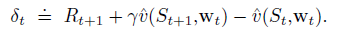
So we can interpret $r_t + \gamma V^\pi(s_{t+1})$ as the TD Target, and we define the TD(0) error as

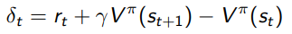
So again, the key here is that we only require $s, a, r, s’$ to compute the TD error and therefore we can be far more efficient with our data.

The TD Learning algorithm 💻

1. $V^\pi(s) \leftarrow 0$

2. Grab a bunch of state-action tuples and …
   1. Sample $s_t, a_t, r_t, s_{t+1}$
   2. $V^\pi(s_t) \leftarrow V^\pi(s_t) + \alpha([r_t + \gamma V^\pi(s_{t+1})] - V^\pi(s_t))$

Properties of the TD Learning algorithm

The TD learning algorithm will give you a different number than the Monte Carlo algorithm, which makes sense

Like with the MC, the $\alpha$ determines behavior

• if $\alpha = 1$, then we update $V$ to the TD target directly, which may cause some oscillation, although this also means that you are doing a bellman backup which as the contraction property.

• If $\alpha = 0$, then nothing changes

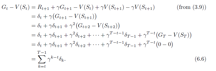
Interestingly, Monte Carlo error is just the sum of TD errors. So that’s why they are the same thing! And in fact, if you “stage” the updates until the end of each episode, TD is equivalent to MC.

• Proof

  

Certainty Equivalence Methods

Here’s an interesting idea…we have a whole toolkit to evaluate policies if we were only given $P(s’| s, a)$. So…can’t we estimate this from existing data?

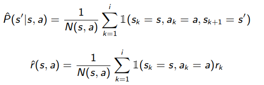
It turns out that this is a good idea. And it’s an unbiased estimator, so it should yield the final policy.

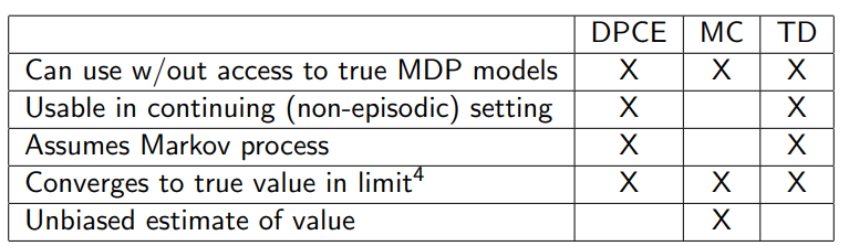
Comparison of methods

Intuition

You can look at the trajectory distribution as a tree

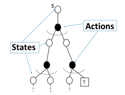
where each black to white node is a sampling process.

Monte Carlo is like shooting a bunch of paths down the tree and taking the average. You’re estimating the expectation across the whole trajectory space.

TD learning is like shooting one single transition. You’re estimating the expectation across transition space, which is far lower dimensional and therefore less high variance.

Aside: Metrics 🔨

We care about the following four properties

1. Robustness to Markov assumption

2. Bias/variance (see below)

3. Data efficiency

4. Computational efficiency

Let’s talk about bias/variance for a second:

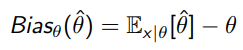
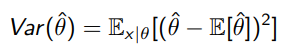
Remember that for an estimator $\hat{\theta}$ to the real value $\theta$, we have

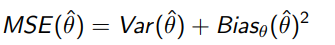
and MSE you can show to be

An estimator is consistent if

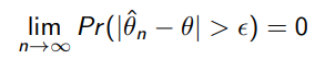
Or, in other words, as you iterate more and more on this estimator, you get arbitrarily close to the real value.

An estimator is unbiased if the average bias is $0$. Here are some critical facts

• an unbiased estimator need not be consistent. For example, $V = G_{i, t}$ is unbiased (because it doesn’t over or under estimate on average), but it is not consistent because it never contracts or converges within an epsilon ball

• A consistent estimator is necessarily unbiased

Metrics applied to Monte Carlo

Monte Carlo is a very naive way of evaluation, but it has some nice properties too.

Bias Variance

tl;dr under some mild assumptions, MC converge to the right value

• First-visit Monte Carlo yields an unbiased estimator of $V^\pi$

• Every-visit Monte Carlo yields a biased estimator of $V^\pi$

• Incremental Monte Carlo properties depend on what $\alpha$ is
  • You can let $\alpha_k(s_j)$ be the $\alpha$ at the $k$th update step for state $s_j = s_{it}$ (so it can vary).
  • If $\sum^\infty \alpha_k = \infty$ and $\sum \alpha_k^2 < \infty$, then the incremental MC will converge to the true value $V^\pi$. (consistent)
  • Example (1/N(s))

    If we let $\alpha_k = \frac{1}{N(s)}$, it will converge. Because every time you visit a state $N(s)$ increments. This yields a harmonic series, so it diverges, but the squared term converges.

Markov

• no markov assumption

Data efficiency

• very data inefficient

• generally, MC is a high variance estimator and requires episodic setting. However, sometimes we prefer MC over dynamic programing if the state space is large and sparse. You can just focus on getting the right $V(s)$ for a set of states that matter, and you can easily get that done through MC, while in TD learning, it is not possible.

Computational efficiency

• Complexity $O(L)$ with $L$ being trajectory length

Metrics applied to TD learning

Bias Variance

• TD learning is a biased estimator and depends on initialization. Why? Well, the TD target can be wrong on average at first. If you inintiaize your $V = 0$, then your target will just be $r$, which is systematically wrong.

• Under the same $\alpha$ conditions as MC, TD learning will converge to the true value of $V^\pi$.

Markov

• exploits MDP property

Data efficiency

• TD learning doesn’t have the episodic assumption, and it is generally lower variance than MC. Exploits markov property, though.

Computational efficiency

• complexity $O(1)$ per update, for an entire episode, it is $O(L)$

Metrics applied to Certainty Equivalence

Bias Variance

• Yields a consistent estimate

Markov

• exploits MDP property

Data efficiency

• we can leverage all our data to make this model, so it is data efficient.
  • unlike all the other methods, we can use this transition model to do off-policy evaluation

Computational efficiency

• For Certainty Equivalence, each update to the MLE model $P(s’| s, a)$, we have $O(|S|^3)$ analytically, and $O(|S|^2|A|)$ for iterative. We have to do this for every update to the model, so it is computationally inefficient.

N step returns

There are two ends of the spectrum: the bootstrap and the monte carlo. They have pros and cons (pretty extreme). Can we get something in-between?

Yes! So we can use Monte Carlo for $n$ steps and use a boostrap estimate for the rest of the steps. This is the intermediate of the bias-variance tradeoff. This is very helpful because variance increases as time goes on. So you’d rather get an unbiased monte carlo estimate near the current time, and then use a biased, low-variance estimate after $n$ steps.

Eligibility Traces

Eligibility traces are ways of unifying TD and Monte Carlo methods. N-step returns are one way of doing this, but there is an even more elegant algorithmic mechanism that has better computational efficiency too.

Conceptually, the eligibility trace is an augmenting factor that gets a bump every time something is relevant, but this bump decays through time. With this “bump” vector, we don’t need to store the past $n$ feature vectors.

Moving from n-step returns

Recall that we define the $n$ step return as follows:

Can we average together different returns? This could give us some nice properties.

Creating the $\lambda$ return (Generalized Advantage Estimation)

The GAE or the $\lambda$ return is the weighted average of n-step returns. Intuitively, we prefer cutting earlier because there is lower variance. But you still want future Monte Carlo to contribute. This yields an exponential falloff summation:

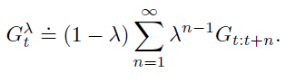
The GAE allows you to create a smoother tradeoff between bias and variance. If $\lambda = 0$, then we have (assuming $0^0= 1$) a standard TD target. As $\lambda → 1$, we get closer to Monte Carlo.

We can use this to train any value function or Q function. But how do we actually compute this term?

$\gamma$ return is a forward method

The $\gamma$ return is still a forward method, like all of TD learning and Monte Carlo. Why is it forward? Well, because you’re looking at future states to update your current state.

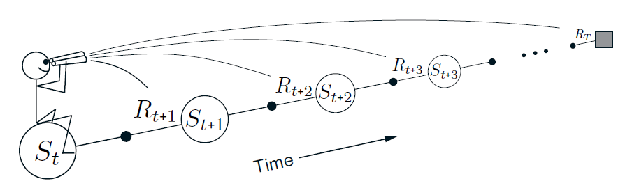
Most critically, you need to know the future in order to update anything. This is a problem for online algorithms, which ideally would like to update as it is executing in the environment.

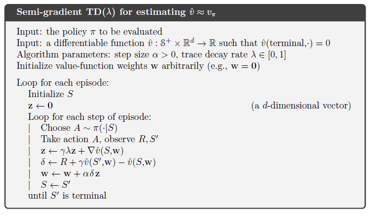
TD-lambda ($TD(\lambda)$) approach

The TD lambda approach proposes using a slightly different method to fit to $\gamma$ return without waiting to the end of an episode. We use something called eligibility traces.

Eligibility trace

The eligibility trace isn’t the hardest concept: it’s something that keeps track of weight updates throughout an episode. It is used because we are doing things without knowing the future states. We add a discount factor to make sure that recently visited states get higher priority

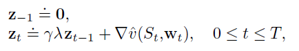
We can interpret this update technique as a backward-facing update, where we are broadcasting current experiences into past states.

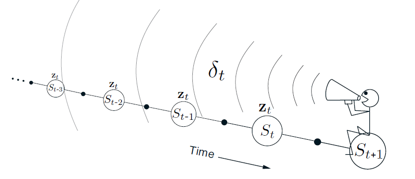
Eligibility trace updates

The eligibility trace tells us which states have been visited and how they contribute to the gradient update. However, they point upwards, i.e. they push the values up if we experience a currently reinforcing phenomenon. However, we can’t just blindly use this update rule

• if we are expecting a reinforcement, we shouldn’t change anything

• if we get an unexpected reinforcement, we should bump up

• if we get an unexpected punishment, we should bump down.

These facts point us towards scaling the eligibility trace by the TD error $\delta_t$.

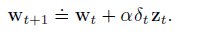
• Algorithm

  

The role of $\gamma, \lambda$

$\gamma$ is the discount factor for the TD error, and it also scales the eligibility trace. This gives some neat properties that we will explore.

If $\lambda = 0$, then the trace is exactly the gradient at this point, scaled by the TD error at this point. In other words, it is the standard one-step TD update. As $\lambda$ increases, more of the preceding states are changed, i.e. given credit for the present state of being.

If $\lambda= 1$, we note that we still scale credit in past states by $\gamma$…which is exactly the monte carlo update. This brings us to an interesting observation: $\lambda$ controls the bias-variance tradeoff

Equivalency to $\lambda$ return

This Eligibility trace algorithm estimates the $\lambda$ return objective without needing an infinite sum or recursive computation.