What’s our main problem?

So in the last section, we were able to compute $V^\pi$ in a few different ways. We could do this by letting the policy run as normal and then averaging the returns.

The problem is that we were only able to evaluate the policy. We really want to derive a policy using similar methods.

An intuitive start is to use the rollouts of $\pi$ to estimate $Q^\pi(s, a)$. But there’s a critical problem: with a determinsitic policy, we won’t be getting sufficient action coverage! We always pick the same action!

Again, remember that if we had $p(s’ | s, a)$ we don’t have any of this problem. In fact, we can arrive at the optimal policy with out any exploration. The problem of exploration is only present in these model-free situations.

How do we intend to solve it?

We will first show how we are to use similar methods as policy evaluation to learn our $Q$. This will yield an on-policy control algorithm that requires data executed from the current policy. We will then show an off-policy control algorithm that can take any arbitrary dataset.

Remember: control is nothing more than evaluation with an additional policy definition step.

Exploration

To start with $Q$, we need to resolve the problem of $Q(s, a)$ learning. We can’t just have a greedy policy running in the environment. Rather, we need to have some degree of exploration.

$\epsilon$-greedy policy 💻

The idea here is pretty simple: there’s an $1 - \epsilon$ chance that we select the greedy action $\arg \max_a Q(s, a)$, and there’s an $\epsilon$ chance of doing a random actin. Therefore, at every state, you can start expand across every action, with a bias on what you think is the best action.

Epsilon-greedy is a key way to juggle exploration and exploitation as we learn our policies from scratch

We often ramp the $\epsilon$ as the agent learns. We start with a high $\epsilon$ and then anneal as the agent gets better.

Boltzmann exploration 💻

You can try something softer and essentially reduce the “hardness” of the distribution

Monotonic guarantees

You can actually show that with $\epsilon$-greedy, the policy still improves monotonically.

Monte-Carlo

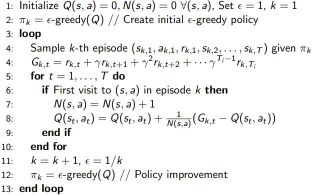
The idea of Monte-Carlo contro is actually pretty easy. In the last section, we talked about how we used count-based methods to derive $V$. Now, we just treat $s, a$ as a unique identifier instead of $s$, and we still use count-based methods

Control with the Monte Carlo Algorithm ⭐

Essentially keep the same count but for $Q$, and we use an epsilon-greedy policy to help with exploration. We continue to extract a greedy policy as we iterate on the $Q$.

Guarantees

So this is a little different than Monte Carlo policy evaluation, where the policy was stationary and you kept you trying to get a better approxmation. In this case, the policy is non-stationary, and you’re not training everything to convergence. Therefore, each $Q$ is not a good estimate of $Q^{\pi_k}$

This procedure might also fail to get $Q^*$ if the $\epsilon$ is too small and we end up getting stuck in a local optimal policy and don’t really explore anything else.

However, we have the Greedy in the Limit of Infinite Exploration (GLIE) condition. According to this, if

• $\lim N(s, a) = \infty$ (all states should be readily accessible)

• $\lim \pi(a | s) = \arg \max_a Q(s, a)$ (epsilon has to ramp to 0)

then these are sufficient conditions for the convergence of $Q$ to $Q^*$.

MC off-policy

We can use MC approaches and importance sampling if you have access to the old policy and the one you’re currently trying to explore. However, importance sampling can be very unstable.

Temporal Difference

Previously, we used TD approaches to evaluate policies. Can we adapt them for control?

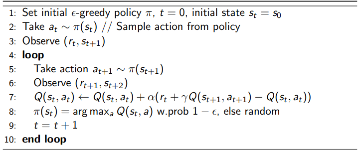
The SARSA Algorithm ⭐💻

So this is very literally the same TD policy evaluation approach. We just need to sample $s, a, r, s’, a’$ where $a, a’$ are sampled from the policy. Note that this requires the additional $a’$

Expected SARSA

You can run SARSA, but instead of using $a_{t+1}$, you can take the expectation over your current policy $\pi$ (more relevant if you’re donig SARSA on a specific policy, not the greedy one)

Properties of the SARSA algorithm

The SARSA algorithm is on-policy, meaning that the data we use must be sampled from the same current policy. This is because we are trying to make $Q^\pi$, and the $a, a’$ must be sampled from $\pi$.

SARSA will converge to $Q^*$ if

• $\lim \pi(a | s) = \arg \max_a Q(s, a)$ (epsilon has to ramp to 0)

• Step sizes $a_t$ satisfy Robbins-Munro sequence, i.e. $\sum a_t = \infty$ and $\sum a_t^2 < \infty$.
  • a good value is $a_t = 1/t$. Intuitively, you can think of this as annealing.

Q Learning

We just saw the SARSA algorithm, which is basically model-free policy iteration that estimates the $Q$ and then improves $\pi$ based on $Q$. Now, this means that the data we use to estimate the $Q$ must come from the current $\pi$, which makes it on-policy. This isn’t very data-efficient.

Instead, we can try to estimate $\pi^*$ while acting under a different behavior policy $\pi_b$, which we call an off-policy RL algorithm.

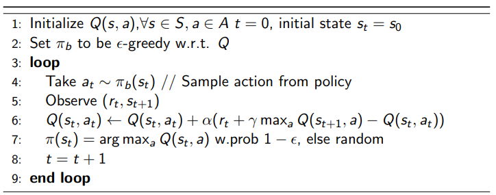
The Q-learning algorithm 💻⭐

Note that there is only one difference: we replace the $Q(s_{t+1}, a_{t + 1})$ with the maximization operation.

Properties of Q learning

If $\epsilon = 0$, the Q-learning algorithm is EXACTLY the same as SARSA, because the $\max Q$ is implicit in the policy. If $\epsilon > 0$, the difference is that the current Q function evaluted by SARSA is the epsilon-greedy policy, not the pure greedy policy of the Q-learner

To converge to $Q^*$, we just need to visit all $(s, a)$ pairs infinitely often and satisfy Robbins-Munro with the $\alpha$. We don’t need to reduce the $\epsilon$ to have $Q^*$.

To converge to $\pi^*$, we just need to make sure that our $\epsilon → 0$.

Why is Q-learning off-policy? Well, the critical part is that we only needed $s, a, r, s’$. These actually don’t depend on any policy. It just means “suppose that I was in this state and took this action, what happens?” This is in contrast with SARSA, which required $s, a, r, s’, a’$. This last $a’$ comes from the current policy, and so the update is bound to the current policy. It’s very nuanced!

In Q-learning, we just imagine that we follow the Q function greedily past this first $s, a, r, s’$. This means that it is off-policy. You can easily plug in data collected from any arbitrary policy and it will learn (although some better than others).

Quick summary about convergences

• GLIE means that all states are visited infinitely many times, and your policy limits to the greedy one
  • Monte Carlo relies on GLIE
  • SARSA requires GLIE
  • Q-learning doesn’t require the greedy limit, but it requires all states

• Robbins-Munro sequence gives us a condition on the learning rates
  • necessary for SARSA and Q-learning

What happens if they break? (Q learning)

If you don’t visit all possible state-actions, you may not convege to $Q^*$. In fact, if you perform Q learning with a Q value initialized to 0 and positive rewards only, on data that is collected by a deterministic policy, the $\max_a Q(s, a)$ will always select the only non-zero value, which comes from the $a = \pi(a | s)$. So, in this case, Q learning actually converges to the data-generating policy