Ways of understanding V and Q

• $V(s) = E_{a \sim \pi} r(s, a) + \sum_s’ p(s’ | s, a)V(s’)$ (this should be true for a converged value function in the tabular world

• $V(s) = E_{\tau \sim p(\tau)}[\sum_i\gamma_ir(s_i, a_i)]$ (this is what the value function is approximating, the average return based on an expectation across trajectories).

• $Q(s, a) = r(s, a) + \gamma \sum_s’ p(s’|s, a)V(s’)$ (this is true for a converged Q function in a tabular world)

• $V(s) = E_{a\sim \pi}[Q(s, a)]$

Q is used for control, V is used for evaluation. They have an intimate connection with each other.

Policy Iteration in an MDP 💻

policy iteration is the gradual creation of a policy in a systematic way that yields a good policy. We do this with a two-step process:

1. make a good policy evaluation of $\pi_i$

2. make a policy improvement based on this policy evaluation and yield $\pi_{i+1}$.

V function (step 1)

Through the bellman backup, you can yield a perfectly accurate $V^{\pi_i}$. This is done for an infinite horizon value of a policy, by default.

But how do you use it?

Q function (step 2)

How do we make a good policy based on policy evaluation? Well, we previously wanted to take argmax over $V^\pi$, but that was too impractical. To help, we need to define a new function in terms of the V function we got in step (1). We call this the Q function:

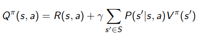
You might recognize this as the inside of the expectation bracket of the bellman backup. In other words,

so as much as we are building $Q$ from $V$, we can just as readily build $V$ from $Q$. They are inherently interconnected.

Intuitively, the Q function means “take action a, and then follow $\pi$ forever”

Now, we propose to let the new policy follow this rule:

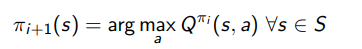
and this is the policy improvement. Now, we will show some critical things about this approach

Monotonic Improvement of policy 🚀

We define a monotonic improvement in a policy by this definition

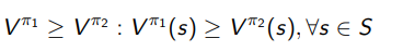
here, again because we are dealing with a tabular environment, we assume that every $V$ is converged.

We will show that the policy improves monotonically if we use the policy iteration algorithm defined previously.

• Proof (fundamental property between V and max Q, then recursion)

  

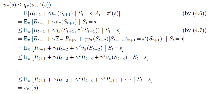
  the reason why the first inequality holds is that we can definitely substitute in $\pi$, and it will be an equality. When we improve over this $\pi$ in policy improvement (see above), we can’t do any worse than that.

  We see here a recursive proof, where we make a rollout of the definition of $v$ over and over until you get to the base case.

Key results from monotonicity 🚀

If the policy stops changing, then it can’t change again. We can show this inductively. Suppose we had $\pi_{i-1} = \pi_i$. Then, we know that $Q^{\pi_{i-1}} = Q^{\pi_{i}}$ (or at least their maximums match). Therefore, if we define $\pi_{i+1} = \max_a Q^{\pi_i}$, we know that

So, if $\pi_{i-1} = \pi_i$, then $\pi_{i+1} = \pi_i$, and the rest inductively follows.

There is a maximum number of iterations of policy iteration: because policy improvement is monotonic and because there is only a finite number of policies, you will eventually converge on the best.

Bellman Operator 🐧

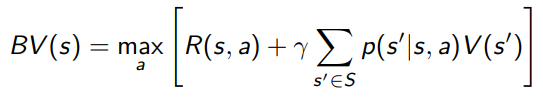
We define the bellman operator $B$ as a function that runs bellman backup on a value function. When we talk about value iteration (below), the bellman operator is defined as

When we talk about policy evaluation in our previous setup, we define the bellman operator as

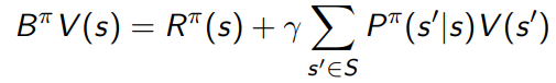
which means that in policy evaluation (above), we can see it as applying the operator repeatedly until things stop changing

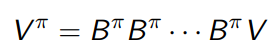
In the next section, we will show some neat things about this operator. Essentially, $V^\pi$ is a fixed point of the operator.

Contraction 🐧

We define a contraction as some operator $O$ and some norm such that $|OV - OV’| \leq |V - V’|$.

Intuitively, if the norm was L2, applying this operator to any vector will shrink it towards some common point. We want to show (below) that the bellman operator is a contraction on the infinity norm.

Value iteration in an MDP 💻

You can think of policy iteration as a slow dance between the policy (implicitly defined in terms of $Q$) and the value function $V$. Again, it’s a dance because you make a future policy from a past policy evaluation. You can think of it as bootstrapping.

But in this process, you have a policy that slowly improves. In value iteration, you ditch the policy altogether. It just doesn’t exist. You immediately try to compute $V^*$, which is the value function of the optimal policy.

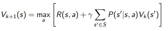
or $V_{k+1} = BV_k$.

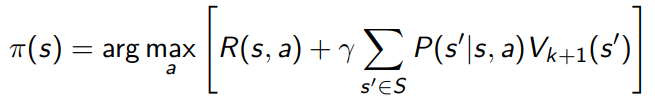
To extract the optimal policy, you just need to do

Value iteration vs policy iteration

Now, this is a common footfall: you might think that value iteration is just policy iteration in disguise. After all, you say, isn’t the right hand side just $\max_a Q(s, a)$? Isn’t this just smushing the two steps together?

Here’s the slight but important difference

1. Policy iteration will compute infinite horizon value of a policy and then improve the policy through that means. This is because we have a policy, even though it’s implicit, it’s still a policy.
   1. we showed that policy iteration yield a monotonically increasing policy, which is enough
   2. this is related to policy gradients, which we will cover later

2. Value iteration never has a policy. You can imagine it as starting from an end state where $V(s') = 0$, and then greedily maximizing $R(s, a)$. This gets us the $V$ for the optimal policy acting on the state $s$ before the end state. Then, imagine moving backwards to the state before $s$. The value iteration step will make the $V$ for the optimal policy acting on the state before $s$, and so on and so forth.
   1. as another way of understanding it: policy iteration there’s a set solution. In value iteration, you’re kinda chasing your own tail a little bit. We actually need to show that the bellman backup is a contraction.

Here’s another way of understanding the difference: with policy iteration, if you pull a $V^\pi$ out of the algorithm prematurely, you can say very little about it. In contrast, for value iteration, if you pull a $V$ prematurely, you can say that it is the optimal value function for $k$ steps, with $k$ being the number of times it’s been run so far.

the tl;dr is that policy iteration is a story of bootstrapping, while value iteration is a story of planning. If you run it long enough, the $V$ will be optimal at any state. Namely, if the environment is ergodic and you need $k$ steps to reach anywhere, then you only need to run value iteration $k$ times.

Will value iteration converge? 🚀

Well, we seek to show that this is true (infinity norm)

• Proof (using properties of maximums and infinity norms)

  

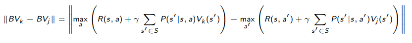
  We use the critical insight that $\max(a - b) \geq \max(a) - \max(b)$. Intuitively, this is true because $max(b)$ is the closest to $a$ that $b$ gets. So we can always do better by sweeping a line.

  This yields the inequality

  $$||BV_k - BV_j|| \leq \gamma \max_a||\sum_{s'} p(s'| s, a)(V_k(s') - V_j(s'))||$$

  And we know that $V_k(s’) - V_j(s’)\leq ||V_k - V_j||$ by the definition of the infinity norm, so we can actually strengthen the inequlaity

  $$\gamma \max_a||\sum_{s'} p(s'| s, a)(V_k(s') - V_j(s')|| \leq \gamma \max_a||||V_k - V_j||*\sum_{s'} p(s'| s, a)||$$

  and the probability collapses to 1, so we get

  $$\gamma \max_a||V_k - V_j||$$

  and we drop the maximum because there are no more $a$ left. So, we get $\gamma ||V_k - V_j||$ on the right hand side, so we conclude that $|BV_k - BV_j|| \leq \gamma ||V_k - V_j||$ as desired.

Is the convergence unique? 🚀

Here, we show the uniqueness of the fixed point

• Proof (simple fixed point properties and contraction)

  We have that $||BV_1 - BV_2|| \leq \gamma ||V_1 - V_2||$ from what we said above. Now, say that $V_1, V_2$ were fixed points. Then, $BV_1 = V_1, BV_2 = V_2$. Therefore, we have

  $$||V_1 - V_2|| \leq \gamma ||V_1 - V_2||$$

  and if $\gamma < 1$, the only way for this to be true is if $||V_1 - V_2|| = 0$, which means that $V_1(s) = V_2(s)$ for all $s$, and the fixed points are equal. Therefore, we conclude that the fixed point of $B$ is unique.

Is value iteration steps bounded? 🚀

We saw with policy iteration that we can only iterate for at most $|A|^{|S|}$ steps before we get convergence. That was because we trained the value function to convergence $V^\pi$ every time. In contrast, with value iteration, we sort of slowly approximate $V^*$. So does the same limit still apply?

It turns out that no, there is no such limit anymore. Intuitively, the value function might “drag” behind and take a long time to converge, even if the greedy policy extracted from it is correct.

• Example

  Take for example a very simple MDP with one state and one action. So policy iteration would converge in one step.

  However, for value iteration, suppose that you start with $V(s) = 0$, and your reward is $r = 1$ with $\gamma < 1$. In this case, after one value iteration step, you get $V(s) = 1$. In reality, it is $1/(1 - \gamma)$, and you would need to iterate for an infinite number of times to get this exact value.

Additional questions to consider

1. Is value iteration going to yield a unique solution?

2. Does initialization matter?

Value iteration as finite horizon planner ⭐

Here, we re-explore the thing we just talked about: value iteration can be seen as a way of expanding our planning horizon by one step every time we run the algorithm.

Let $V_k$ be the optimal value if making $k$ more decisions. Then, let’s initialzie $V_0(s) = 0$ for all states. Now, we run value iteration

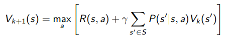
Now, you see how we can integrate one more time step into $V_{k + 1}$ because we consider this last $V_k$ on top of the current reward. So there’s this branching out of states. It’s kinda cool!

The saga of $V^*, V, V^\pi$ (and the greedy policy)

To be clear, $V$ can be any vector of size $|S|$. Now, there exists some $V^*$ which is the best possible value function for an environment. Similarly, there exists some $V^\pi$ for every policy that accuragely describes the return of the policy.

For $V^*$ and $V^\pi$, they are fixed points of the bellman backup and therefore must follow $V^* = \max_a(r(s, a) + \sum_{s’}p(s’ | s, a)V^*(s’))$, and $V^\pi = E_{a\sim \pi(s)}[(r(s, a) + \sum_{s’}p(s’ | s, a)V^*(s’)]$ respectively.

For $V$, no such rule exists. So you can’t write out any relationship that $V$ satisfies. But you can use $V$ in a policy! Just do a greedy selection

Now, we note that for the greedy policy, we have $BV = B^\pi V$because the policy is inherently greedy. But be careful—for any other $V’$, you have $BV’$ pushing towards $V^*$ and $B^\pi V’$ pushing towards $V^\pi$, which is the value of the greedy policy based on $V$, an arbitrary vector.

the tricky part is that $V$ generates $\pi$, which has its own $V^\pi$ that can be very different from $V$.

Reasoning about optimality

Optimality is defined as some $\pi^*$ where $V^{\pi^*}(s) \geq V^\pi(s)$ for all $\pi$ in the environment. If you apply $\pi^*$ to another environment, does the same condition hold for the real vaue function? If so, the optimality still holds. Otherwise, it doesn’t. Linear shifts and positive scales in value functions do not change optimality.

Optimality with shifts in rewards and horizon

• On an infinite horizon, adding a constant $c$ to all rewards does not change optimality. You can prove this by writing out what $V$ is for every $\pi$, and you see that they are all shfited by a constant number (an infinite sum)

• On an infinite or finite horizon, multiplying a constant $c$ to all rewards does not change optimality as long as $c$ is positive. This is because you can factor out a $c$ from any expression of $V$. However, do note that if $c < 0$, then we negate the value, and if $c = 0$, then all policies are optimal

• On a potentially finite horizon (presence of terminal states) adding a constant $c$ to all rewards may change behavior. This is because certain states may “die” first, yielding a shorter summation of discounted $c$ (i.e. $\sum_n^N \gamma^n c$ where $N$ is finite. As such, we may add a value to each $V(s)$ that depends on $s$. Intuitively, this is true because if you add more meaning to life, then we might try living longer before doing anything risky that could end it.
  • simple example: one state with negative reward, and terminal state. With negative reward, optimal policy terminates immediately. Add something that makes the reward positive, and the agent will choose to stay.

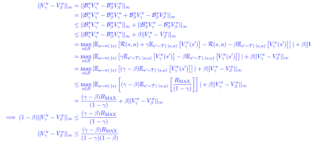
Impact of discount factor on value 🚀

Claim: for any $\beta < \gamma$, we have

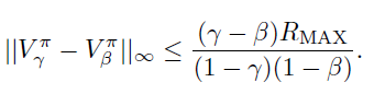
which effectively means that we can bound the differences in the true value.

• Proof (adding and subtracting, recursive bellman)