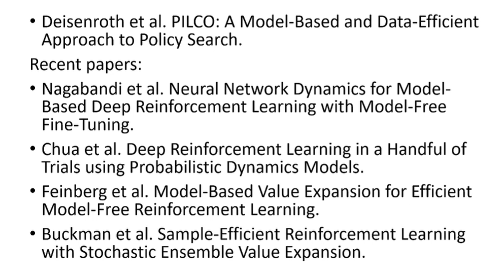
• Additional reading

  

  

  

What models do you learn?

There are many ways of learning a model. Here are the three most popular

• neural network (learn $p(s’|s, a)$, $r(s,a)$)

• parameters to a physics model (more inductive bias baked in)

• hardcoded model (things like games, where every move has certain rules)

In the last section, we saw some ways of optimizing over a known model. That’s fun, but we can’t assume that we can just pluck a working model out of thin air. How do we effectively learn a world model? Sometimes, this goes hand in hand with effective control.

Learning the Model

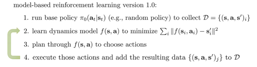
The basic version

1. run policy to collect data

2. fit dynamics model

3. plan through dynamics model a sequence of actions $a_1, …, a_n$ to execute.

What can go wrong? Well, the model can’t predict what it hasn’t really seen before. Therefore, it may not generalize very well, especially to dangerous states that are generally not seen.

You need to have a good base policy that explores very well. This approach works the best if there aren’t too many parameters.

Improving distribution shift

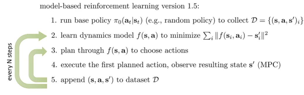
We can improve this paradigm by just improving the model as we execute things online

this is like DAGGER but we are learning a model, so we don’t need to use any supervision.

Model Predictive Control

Even if we have a good model, there still exists small inconsistencies or even just unpredictable randomness. To deal with this, we use a technique called model predictive control.

Right now, the problem is that we have a horizon $n$ that we execute blindly from the controller. Can we somehow replan every step? We can’t just make the horizon 1, or else we get a greedy policy. We just need to keep the horizon, execute one step, and plan again with the new observed state. This approach is called Model Predictive Control.

The more we replan, the less perfect the plan needs to be. We can use shorter horizons, for example . But the big con is the computational cost goes up.

Uncertainty in model-based RL

Model-based learner typically performs worse than model-free learning. First, the iterative data collection process means that we start with a low amount of data, and this data is low quality. Neural networks can struggle with overfitting on this data. And this overfit model can often be exploited by the planner. To help with this problem, we need to look at uncertainty.

There are two types of uncertainty: aleatoric or statistical uncertainty, which is natural noise. If you collect more data, this may not go down. The other type is epistemic or model uncertainty, which will go down if you collect more data. You can always improve epistemic uncertainty.

In this low-data regime, it’s important to impose a measure of data uncertainty. You should only take actions where we think we’ll get high rewards in expectation (WRT the uncertain dynamics). This reduces the chances of doing an action where there exists some potential dynamics that leads to a high-punishment situation

Bayesian Networks

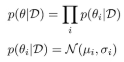
Being uncertain about the model means being uncertain about the model parameters, $\theta$. The uncertainty is therefore $P(\theta | D)$. Normally, you can calculate $P(D | \theta)$ through normal likelihood, but to compute the other way around, you need to marginalize across $\theta$, which is intractable.

Instead, we could use a Bayesian neural network which keeps a distribution over each weight. Commonly, we assume that each weight is independent and a gaussian.

Bootstrap Ensembles

Well, you can just train a bunch of neural networks. When the samples are in-distribution, they will most likely agree. But out of distribution, they often disagree.

Formally, this is like estimating your posterior with a mixture of dirac deltas

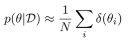
We can train each model on $D_i$ which contains the same number of datapoints as the original dataset $D$, but it is sampled with replacement from $D$. Although, in practice, with SGD and random seeds, we don’t even need to do the random sampling

Planning with Uncertainty

So suppose that we’ve trained an uncertainty-aware model. How do we use it?

We can still use all of our existing planning methods. However, we just need to sample across the model parameters as follows:

1. Sample a $\theta \sim p(\theta | D)$ (amounts to picking one of the models)

2. Sample $s_{t+1}$ from chosen model

3. Calculate $r$ from chosen model

4. Do steps 1-3 to get an estimate of the average reward

There are also other more complicated ways of estimating rewards from our parameter distribution. The key realization here is that the average of the ensembles can let us know about certain risky states, even if most of the ensembles think that something is safe. As long as there’s a possibility of something terrible happening, we will see it in the average.

Model-based RL with images

So far, model-based RL has mostly stayed in lowdim control. When we are dealing with images, we are dealing with a POMDP. The observation may not capture all of the information of the underlying state.

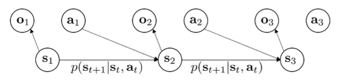
However, model-based RL with images allow us to segment the image generation $p(o_t | s_t)$ and the dynamics $p(s_{t+1} | s_t, a_t)$. In this case, $s$ is a latent space.

State space models

We learn three models

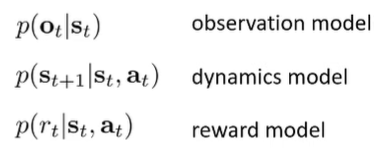
We can treat $s$ as a latent variable, which creates this objective

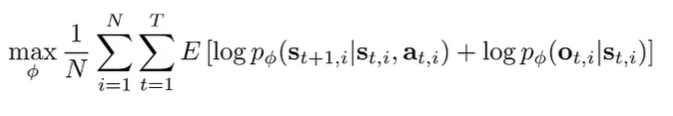
The expectation is over $(s_t, s_{t+1}) \sim p(s_t, s_{t+1} | o_{1:T}, a_{1:T})$. This is derived by just the simple maximum likelihood objectives over the state marginal distribution (there is no inference here yet). The posterior state marginal is intractable, but we can use a variational technique to approximate the posterior. There are also different types of posteriors you can learn

• $q(s_t, s_{t+1} | o_{1:T}, a_{1:T})$: full smoothing posterior, more accurate but more complicated

• $q(s_t | o_t)$: single step encoder, simplest but less accurate

The more partially observed the environment, the more you want to have a full smoothing posterior.

Learning directly in observation space

You can also learn directly in the observation space by training $p(o_{t+1} | o_t, a_t)$. This is definitely more possible with advances in image models. You may want to include more history too.