• Additional reading

  

  

From Planners to Policies

In a previous section ,we talked about classic control (MPC, LQR, etc), which use world models to optimize an open loop sequence of actions. Open-loop planning means that we can’t create any reactive decisions, which severely limits the policy. Can we make a closed-loop policy using information from the world model?

Direct Gradient Optimization

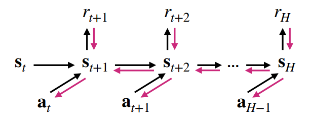
If we assume that everything is deterministic and assume that the model is perfectly correct, then the rollout is just a computational graph. Therefore, you can just backpropagate and do gradient ascent against rewards.

The actual algorithm looks a little like this

1. Fit the model

2. optimize against the model

3. collect more data using the trained policy, use it to fit the model again

4. repeat steps 1 - 3

Pros and Cons

This technically works, but it doesn’t work well. It’s an ill-conditioned optimization problem.

• mistakes can be exploited

• uneven sensitivity

• no dynamic programming approaches (so it’s hard to optimize long horizons)

Connection to policy gradient

Here’s an interesting connection: the policy gradient and the direct model gradient (see above) are estimators of the same thing, although the former doesn’t require a knowledge of the dynamics

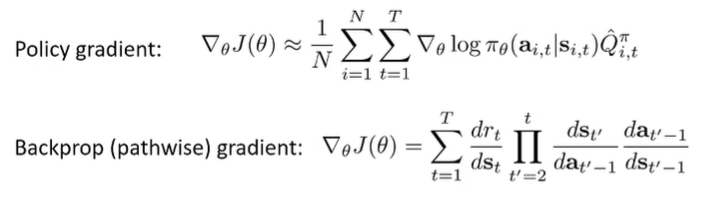
In fact, the policy gradient is likely more stable, because it doesn’t require jacobian multiplication. Therefore, you can actually use REINFORCE on the computation graph, which can yield better results.

Derivative Free Algorithms

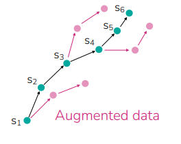
The big idea is that model-free approaches can need a lot of data. What if we use a model to generate samples?

The general philosophy is this: take a trajectory, and try different partial trajectories from all the states by running it through the model. This is just augmentation.

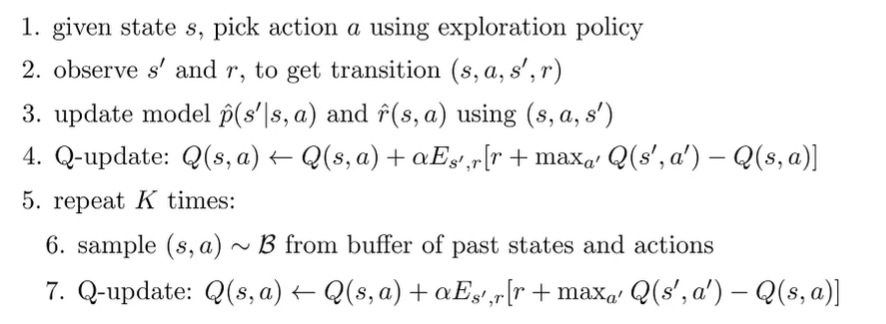
Dyna

The idea of Dyna is basically the following

1. Explore online (using exploratory policy)

2. update world model using explored experience

3. Learn with Q method with a mixture of explored experience and imagined experience, where you sample $s, a$ from buffer of past statess and infer $s’$.

• Algorithm

  

Modern versions of Dyna use similar ideas, although here are some common differences

• Sample $s$ from buffer and $a$ from current policy

• Take multi-step rollouts from the real state $s$ (shorter means that you don’t have compounding errors, but you still have multi-step data

Three algorithms include Model-Based Acceleration (MBA), Model-Based Value Expansion (MVE), and Model-Based Policy Optimization (MBPO)

Local Policies

LQR with Local Models (LQR-FLM)

In LQR, we used $df/dx, df/du$ to solve for locally optimal policies. However, we can fit these values around current trajectories. We do this by creating an empirical estimate of the derivative, and fitting the linear function to this empirical estimate. More specifically, we fit $p(x_{t+1} | x_t, u_t)$ using linear regression such that $p(x_{t+1} | x_t, u_t) = N(A_tx_t + B_t u_t + c, N_t)$.

With the dynamics estimate, we can use iLQR to get the local controller based on this empirical estimate. iLQR gives you a local policy that gives you $\hat{x}, \hat{u}, K, k$ such that $u = K(x - \hat{x}) + k + \hat{u}$. Recall that $\hat{u}$ is your best guess, and you refine it based on this dependence. But how do you use this for control?

• You can just use $\hat{u}$, but this is open loop and doesn’t correct for deviations

• You can use the definition of $u$ (see above), but this actually might be a bit too good. You need some variance in the policy so you get different states for your $df/dx, df/du$ fitting process.

• Add noise such that all samples don’t look the same (basically epsilon greedy), and set $\Sigma_t = Q^{-1}$, where $Q$ is the Q function matrix with respect to $u$. Don’t worry about this too much; it’s just a neat little trick.

Because the dynamics are only locally correct, we need to constrain the action distributions. Note that this looks very similar to policy gradient, where you’re collecting data using $p(\theta)$ and you’re constructing $p(\theta’)$. If you want the estimate to be correct, you need $\pi_\theta$ to be close to $\pi_{\theta’}$. And because the new distribution comes from a linear controller, the KL constraint $D_{KL}(p(\tau) || \bar{p}(\tau))\leq \epsilon$ is actually not hard to do, because the KL constraint is linear-quadratic. You can just modify the cost function and add a term that penalizes how far away we are from the previous policy.

Global Policies from Local Models

Guided Policy Search

The high-level idea is to learn local policies (like LQR-FLM) for different situations, collect data, and train a general policy through supervised learning.

Generally, the algorithm is as follows

1. optimize local policy WRT a regularized cost function (the cost function that is regularized based on distance to the current master policy $\pi_\theta$

2. Use samples from local policy to train $\pi_\theta$

3. Update cost function with the new $\pi_\theta$, repeat

Distillation

This actually touches on a larger theme of distillation. A collection of models often do better than single models, but we can often “distill” the knowledge gained by model collections into a smaller model, for lightweight test time running. You just do this by using the ensemble predictions as soft targets (instead of one-hot). Intuitively, the soft distribution gives us more information than hard targets.

We can also just train the policy on a bunch of planner rollouts.