PROOF TRICKS

For bellman backup, think:

• contraction inequality $||BV_1 - BV_2|| \leq \gamma ||V_1 - V_2||$
  • if you can get the same bellman operator under an infinity norm, you can use the contraction inequality

• fixed point uniqueness and property that $BV^* = V^*$.
  • whenever you see $V^\pi$ or $V^*$ think: can you benefit by rewriting it as $B^\pi V^\pi$, $B^*V^*$ because now you can write out the recursive form too.

• the direct definition of the bellman backup. This one is the hardest to use, but sometimes you need to get into the nitty-gritty. This is helpful if you have element relationships, which aren’t covered really well in the infinity norm contraction inequalities

• remember that V is an expectation over trajectories, as well as Q

• remember that a converged V and Q can be written recursively. This is particularly useful if you consider rewards or discounts, as they show up in the recursive formulation

• if you see that something is a fixed point , then it is at the optimality for that bellman backup (it goes the other way too).

What do we want?

So in this setup, we know a model of the world (transitions, rewards, etc). And with this, we want to formulate a good policy.

More than that, we want to evaluate how well a policy does, which is known as policy evaluataion. Typically this involves a $V$ funciton. More on this in a second.

Markov Processes

Remember that a markov process is any process whose future is independent of the past given the present. For all our discussion, we will consider discrete states and actions. This is why it’s know as a tabular setup.

Markov Assumption

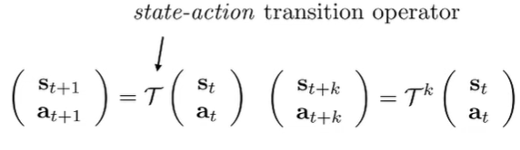
An RL environment is just a Markov Chain. It contains a state space $S$ (can be discrete or continuous) and a transition operator $T$, which represents $p(s_{t+1} | s_t, a_t)$ (it may or may not include $a$). In RL theory we talk a lot more about what this is

The markov assumption is that the future is independent of the past given the present. In mathematical terms,

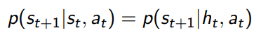
Now, the state doesn’t necessarily need to be one timestep. In reality, it can be multiple because sometimes change is a necessary part of state.

Markov Chains

If the transition is defined by an operator, you can push forward in time by raising the operator to a power

And the question becomes, does $\mathcal{T}$ have stationary distributions? (i.e. $\mathcal{T}\mu = \mu$) If the chain is ergodic and aperiodic, this is indeed the case, as shown in classic Markov chain analysis.

Importance of stationary distribution

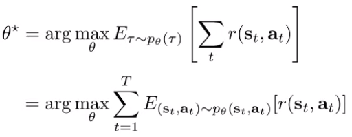
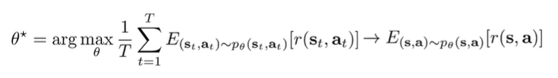
The RL objective is the expectation across the state-action marginal at time $t$ in every step.

However, computing $p_\theta(s_t, a_t)$ is not very practical because of inference costs. However, if we assume infinite horizon, we can make the assumption that the stationary distribution cominates the summation, meaning that we only need to take the expectation across the stationary distribution, something that is easier to do.

Markov Reward Process (MRP)

Definitions

A markov chain is just that: it’s a situation that evolves over time. But we care about rewards. So, we can add rewards associated to each state $R(s)$, as well as a discount factor. The smaller the factor, the more we care about the here and now. For finite horizons, we can just use $\gamma = 1$.

There are still no actions, so it’s like a machine that you pull the crank, watch the marbles bounce around, and collect your reward.

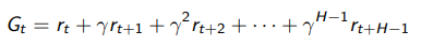
We now need to consider a horizon $H$, which is how long we collect rewards. It can be infinite, or it can be finite. Across a horizon we get a Return $G_t$ which is the discounted sum of rewards from time $t$ to end-of-horizon. This is single-rollout:

Now, suppose that we wanted to know a general truth about a state. Well, we define the state value function $V(s)$ as the expected return

Horizons

We can have an infinite horizon task. In this case, your $\gamma < 1$, or else you might get infinite reward. For finite horizon tasks, you can have $\gamma \leq 1$, because your rewards will always be finite. In general, if you have an episodic structure, you need to be careful that the agent is getting the information that it needs before it resets.

Computing the value function

If you think about it, the value function must satisfy the following condition

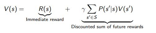
this shouldn’t be a surprise; it’s just how $V$ is defined, as the discounted sum of rewards. Here, this isn’t a function; $V$ is a true value.

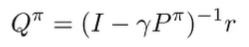
Analytic solution for V

Now, in discrete space, we can vectorize it

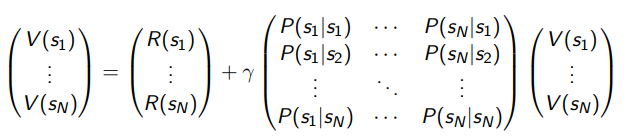
and essentially express $V = R + \gamma PV$. Therefore, we can solve algebraically that

We can show that $(I - \gamma P)$ is invertible, but this process is not efficient. It requires taking a matrix inverse of size $|S|\times |S|$, which is $O(|S|^3)$.

Iterative solution for V

We can improve efficiency by doing an iterative solution that uses dynamic programming. It’s actually pretty straightforward. You just use the old $V$ to compute the new one!

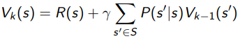
Now, this only takes $O(|S|^2)$ complexity. The iterative solution we will come back to later, as it is the backbone of many algorithms.

Markov Decision Process (MDP)

The MDP just adds actions into the mixture. You can think of actions as just expanding the state. For every action, there is a separate transition matrix. In other words, we care about $P(s’ | s, a)$ now. We also care about $R(s, a)$.

Harnessing the Policy

But how are we supposed to say anything about the MDP if we don’t know what actions to take? Well, the solution is to have a policy that computes $P(a | s)$.

An MDP with a policy just becomes a markov reward process. Intuitively, this is true because if you have someone providing the actions, you just have to pull the crank and let the rewards come out. Concretely, we formulate an MRP where

and

Bellman Backup ⭐

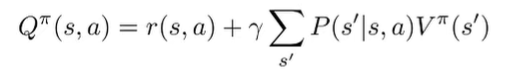
With this conversion, what does the value function look like under an MDP? Well, we can just substitute in our definitions above into the iterative solution:

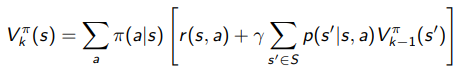
Essentially, the inside of that outer bracket just assumes that we take a certain action, and if we assume that we take a certain action, it’s just exactly the MRP iterative solution to $V$. But we need to take the expectation across the policy because the policy decides which action to take.

We call this equation the bellman backup, and it is critical to Policy Evaluation!

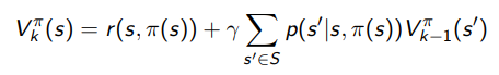
Of course, if the policy is deterministic, the update becomes

For Q functions, the backup just puts in $a$ where the $\pi(s)$ is above.

Towards control in an MDP

Once we have a good $V$, then to find the best policy, we just do

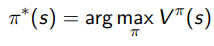
Now this is easier said than done, and we will talk about how we might do this. We call this policy search. We could just search the number of deterministic policies, but this is really, really bad as there are $|A|^{|S|}$ policies.

Here are some facts about infinite horizon problems. The optimal policy is

• deterministic

• stationary (doesn’t depend on time)

• not necessarily unique

Simulation Lemma ⭐

Suppose that you had a simulation of a system with rewards and transitions being $\epsilon$-similar.

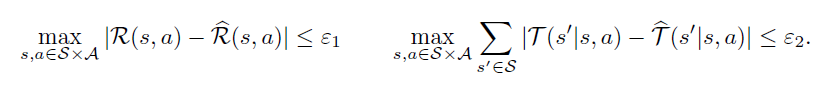
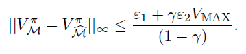
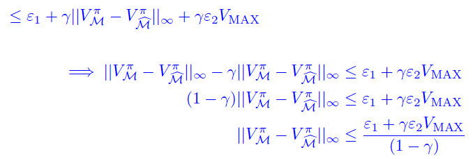
Can you say anything about how the value functions will be different? As it turns out, yes! You can show that

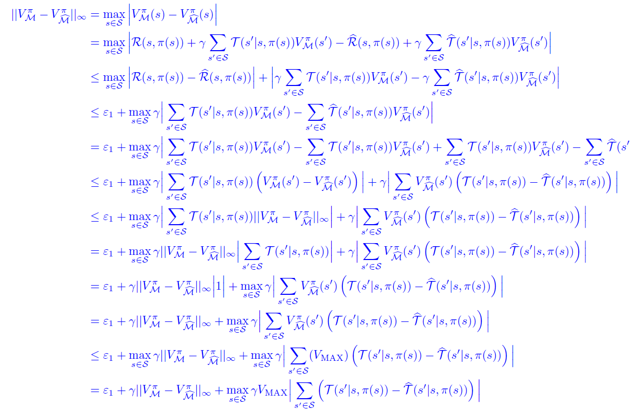
• Proof (recursive rollouts)

  Your spider senses should be tingling: you need to do a rollout to expose the rewards and the transitions so you can pull them into the epsilon bounds

  (it gets a bit cut off but the point should be clear)

  

  

Rederivation from vectors and concentration inequalities (From CS 285)

☝

This is from CS 285 Berkeley. Personally it’s a bit more confusing so I’ve left it here as a collapsible section

Expressing P’s and Q’s

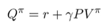
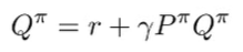
Can we relate $P$ to $Q^\pi$. We have the bellman equation

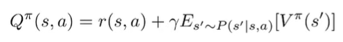
which means that we can write this in vector notation

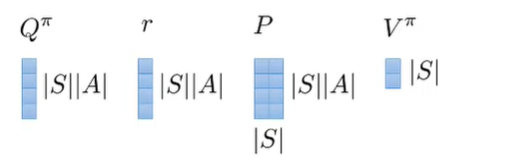
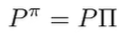
We can also express $V$ and $Q$ in vector notation because $V$ is the expected value of $Q$

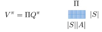
This $\Pi$ is a probability matrix but it’s actaully sparse. It’s only non-zero where the $(s, a)$ in the column matches with the $s$ in the row, because the $V(s)$ uses the same $s$ as $Q(s, a)$. The bellman backup we can write in terms of an $|S||A|\times |S||A|$ sparse matrix. The sparsity comes from the fact that maybe not all states are reachable from other states

which means that we can define this transition matrix as

Combining these two pieces of knowledge, we get

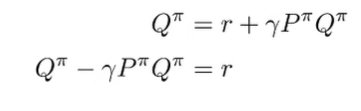
which means that

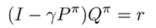
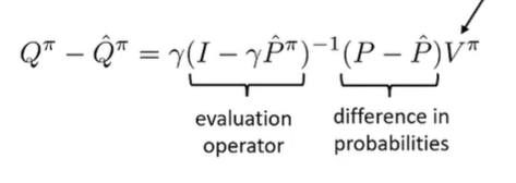
which means that we can show how errors in $P$ can propagate to errors of $Q$. And this goes the same for

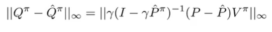
Defining the difference

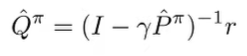
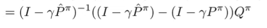
The simulation lemma tells us how a Q function in the true MDP differs from the learned Q function

How do we prove? Well, we can use the previous definition

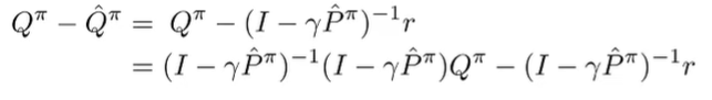
(the second line just adds an inverse and a non-inverse, which cancels out

We replace the $r$ with $(I - \gamma P^\pi)Q^\pi$ using our definitions of Q and P.

condensing.

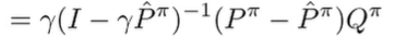
Grouping like terms and canceling things.

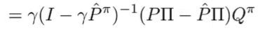
We use the previous identity developed

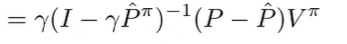
and we use the definition of $V$

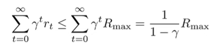
Infinity norm vector transformation lemma

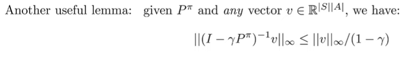
Intuitively, if we let $v$ be the reward, then the Q function (see definitin of Q function in terms of $r$) can’t exceed the true reward by more than $\frac{1}{1-\gamma}$.

👉

Sidenote: the reason why we see a lot of $\frac{1}{1-\gamma}$ is because we have infinite sums where $\sum^\infty \gamma^t c = \frac{c}{1-\gamma}$

The proof: we start with

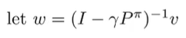
which means that

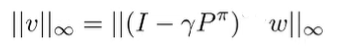
and from the triangle inequality, we get

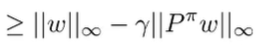
We know that the infinity norm of $P^\pi w$ is less than $w$ because $P^\pi$ is a stochastic matrix, meaning that each term is at most $1$.

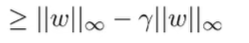
and this gets us

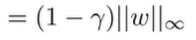
which means that

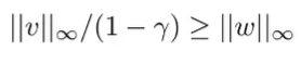
and remember that $w$ is exactly the definition we are looking for.

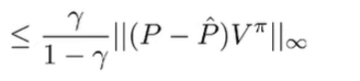
Assembling the lemmas

We can plug in $v = (P - \hat P)V^\pi$ into the infinity norm lemma

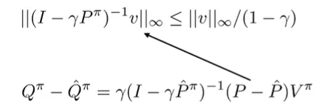
From the simulation lemma, we can put infinity norms around the terms to get

And combining these things together, we get

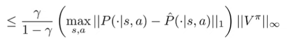
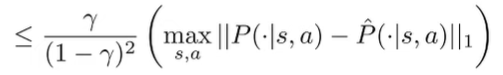
Now, we’ve related the difference of Q to the difference of P. Can we somehow get rid of this $V^\pi$?

Well, the matrix-vector product is less than or equal to the product of the largest entries. This is a pretty crude bound, it it works

And now, we can use our concentration inequalities. First, we bound $V^\pi$

We can assume that $R_{max} = 1$ for simplicity sakes.

And we use the concentration inequality over discrete values

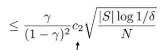
which means that we get

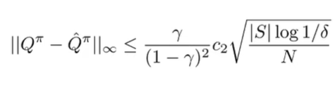
Therefore, we get that more samples means lower error, at the rate of $\frac{1}{\sqrt{N}}$. The error grows quadratically in the horizon (the larger the $\gamma$, the larger the error), which means that each backup accumulates error.

Simple implications

What about the differences between optimal Q functions? Well, we can us can identity

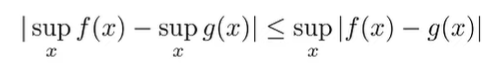
(the differences of maximums is smaller than the maximum of differences)

which is nice!

But what about the policies? Well, we can do the old subtract-add trick, and then the triangle inequality. Then, we can use the previously derived bounds to get

Bellman Residual Properties

A bellman residual is basically what changes during a Bellman update: $(BV - V)$ or $(B^\pi V - V)$. This is the objective that we are optimizing for in value and policy iteration when we update the value function.

Residual is an upper bound to value fit 🚀

Here, we want to know if we can see how close we are to convergence to any policy $\pi$ and any value function $V$, just by doing one bellman backup.

To do this, we want to show that $||V - V^\pi|| \leq \frac{||V - B^\pi V||}{1 - \gamma}$.

Here is the proof

• Proof (using triangle inequality and bellman properties)

  

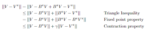
  And we can just move things around to get the desired value.

The exact same proof follows for showing $||V - V^*|| \leq \frac{||V - BV||}{1 - \gamma}$; just replace the symbols.

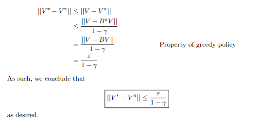
Bounded residual means closeness to optimal value 🚀

Here, we want to know that if you take any value function $V$ and make a greedy policy $\pi$ from it, can we say anything about the value of this greedy policy in relationship to the optimal value?

Mathematically, let $\epsilon = ||BV - V||$. Then, we can show that

• Proof (using previous result and triangle inequality)

  

  And once we get to this point, the property of absolute values is enough to show the desired inequality.

Tighter bounding 🚀

If you assume that $V^*(s) \leq V(s)$ for all $s$, then you have

where $\epsilon = ||BV - V||$.

• Proof (previous result and additional assumption)

  We know that $V^* > V^\pi$, so the vector difference is always non-negative. Therefore, from the additional assumption, we can create the following proof:

  

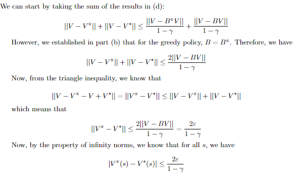
Simpler sufficient condition 🚀

While it may be possible to satisfy the condition of $V^* \leq V$, it requires knowing $V^*$, and that is a strong assumption. Instead, we can show that if $BV \leq V$, then $V^* \leq V$ which allows us to use the tighter bound.

• Proof (backup definition and induction)

  Base case: $BV < V$. Inductive case:

  

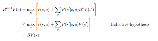
  which means that $B^{k + 1}V \leq V$ (using the base case to make this final conclusion).

  With this shown inductively, we can now move to say that $\lim_k B^kV \leq V$, and we know that $\lim_kB^k V = V^*$. So, we have $V^* \leq V$, as desired.