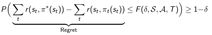
Regret for MDPs

Regret is pretty easily formulated. You can use a probabilistic approach and say that your regret won’t exceed a certain bound with probability $1 - \delta$.

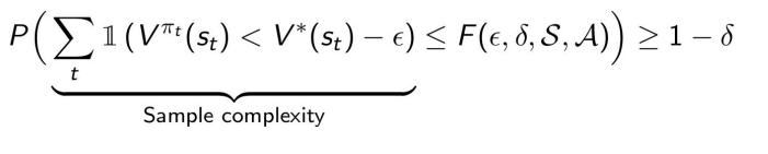
PAC for MDPs

An RL algorithm is PAC if, with probability $1 - \delta$, we have $a_t$ $\epsilon$-close to $a^*$ for all but $N$ steps, where $N$ is a polynomial function of $|S|, |A|, \frac{1}{1 - \gamma}, \frac{1}{\epsilon}, \frac{1}{\delta}$.

We can also say that $V^\pi(s_t) \geq V^*(s_t) - \epsilon$ for all $s_t$; it says the same thing.

Intuition

Intuitively, we can recall the PAC for bandits means that we pick actions whose average reward is within $\epsilon$ of the optimal arm’s average reward. Here, we are doing something similar: we assume that there is some sort of optimal action quantified by $Q^*$, and we just pick $a_t$ that is $\epsilon$ close in $Q^*$.

Not all algorithms are PAC: a greedy algorithm may settle on something suboptimal outside of the $\epsilon$ and yield an infinite $N$.

Deriving PAC

Suppose that you had a simulation of a system with rewards and transitions being $\epsilon$-similar.

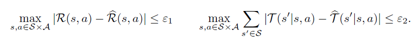
These bounds you can get from Hoeffding’s inequality. Now, with these bounds, you can use the Simulation Lemma (see tabular learning section for proof) to get this

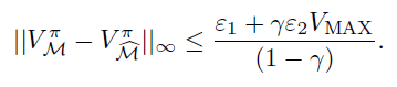
And this would be related to your PAC bounds. If the right hand side becomes a polynomial in the aforementioned terms, then the particular algorithm is PAC.

Optimism in MDPs

Model-Based Interval Estimation with Exploration Bonus 💻

This algorithm, MBIE-EB, uses certainty equivalence methods to estimate the environment rewards and transitions. Then, we add a reward bonus based on the number of states explored.

• Algorithm

  

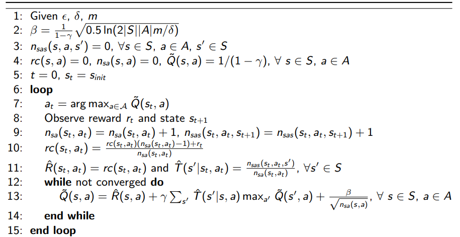
MBIE-EB is a PAC algorithm, although the bound on $N$ is very loose and often too large to be meaningful.

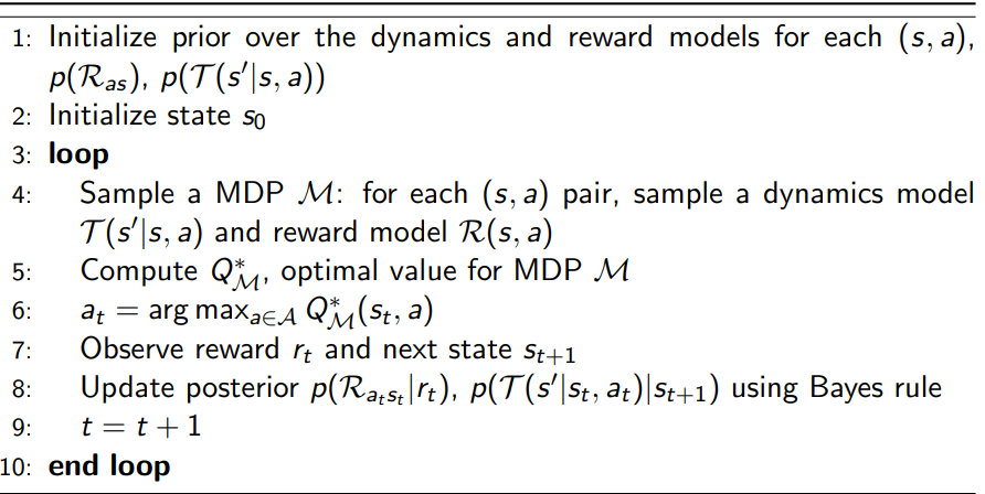
Bayesian MDPs

In the bandit setting, Thompson sampling consisted of sampling parameters for a distribution and then computing the argmax. You can do the same thing with MDPs!

You sample an MDP at each transition (or every episode), compute the Q function, and then act greedily with the Q function. The “parameters” is just the MDP parameters, because it defines the Q function that you use for control.

As you run this Q function on the selected distribution, you update the relevant MDP estimation parameters

• Algorithm

  

Generalization and Function Approximation

Optimism

MBIE may not work out of the box because counting isn’t useful for sparse states. Instead, you can consider adding adding a reward bonus that looks like a real count-based optimism component. In reality, it is a pseudo-count.

Even so, optimism in MDPs create a huge boost in performance!

Thompson Sampling

The naive implementation requires a model and a sampling over MDPs, which is usually intractable. Instead, we can just train $C$ DQN agents using bootstrapped samples from a dataset. Then, for every episode, we sample a Q function and act by the Q function for an episode.

This is more meaningful than randomly sampling an MDP and making a Q function every step, because you can imagine this as selecting a “life philosophy” and acting by it for a while

Where is the research now?

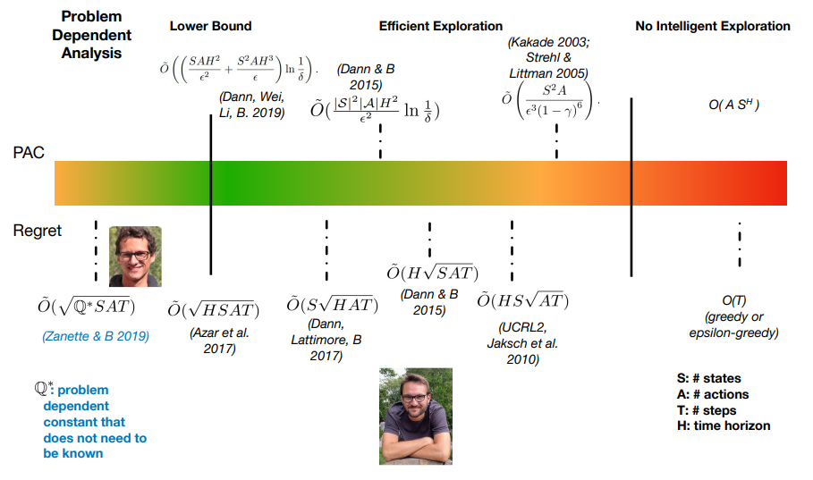
We try to create meaningful lower and upper bounds to performance metrics like PAC and Regret. Above is a graph of bounds that have been discovered.