Linear Analysis

We can use a feature vector to represent some state $s$. As the most degenerate feature vector, we can use $\delta(s)$, which is a one-hot vector. (more on this later).

With the feature vector, we can approximate the value with some $w$

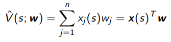
which means that with an MSE objective function

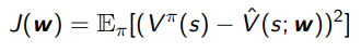
the weight update is

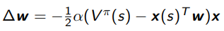
But you don’t have $V^\pi$. So…we make do an approximation.

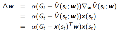
Monte Carlo Value Function Approximation

We can just approximate $V^\pi$ with $G_t$ and get

Temporal Difference Value Function Approximation

We can also just use TD(0) as the $V^\pi$ approximation.

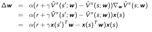
This is a little weird, because we’re invoking the function twice. The key observation is that we are only taking the derivative through $V(s)$, not $V(s’)$ or else we run into some issues.

There are three approximations in TD learning

1. sampling (sampling s, a, r, s’)

2. bootstrapping (the TD part)

3. value function approximation (non-tabular)

Convergence of Linear Policy Evaluation

We know that the bellman backup is a contraction, but this is only based on a perfectly accurate function. In reality, if you’re not in the tabular realm, you can’t say anything about $|V_\theta(s) - V^*(s)|$ because the optimization process is another projection, and this projection in L2 space can actually lead to an expansion in the infinity norm space. So you have to be careful!

Finite state distribution

Define $\mu(s)$ as the probability of visiting state $s$ under policy $\pi$. This is a finite horizon task. Note that it doesn’t use the markov property anywhere, so it works for monte carlo.

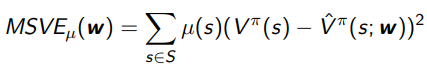
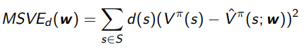
MSVE-$\mu$

We define the mean-squared error MSVE as

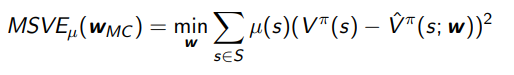
For Monte Carlo policy evaluation, it converges to the minimum MSVE

Stationary distribution

A stationary distribution $d(s)$ is defined as the distribution of states under $\pi$. This is a property of any markov chain: if you set off a swarm of robots in the chain, eventually their populations would stabilize. This is $d(s)$.

Because of the markov chain and the markov assumption, the stationary distribution satisfies this balance equation.

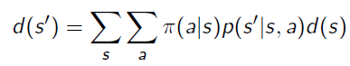
which sort of makes sense. We’re saying that the distribution over $s’$ is the same as the expected transitions of all its neighbors.

MSVE-d

The MSVE-d is the same as MSVE-$\mu$ except that we use this stationary distribution.

For TD policy evaluation, it converges to a scaled version of the minimum MSVE-d as follows:

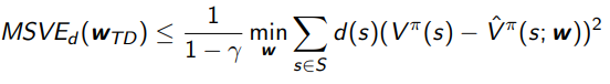
The larger the gamma, the worse the upper bound.

Linear Control

Control using function approximations is basically just approximating $Q^\pi$ and using the same policy-evaluation + policy improvement approach.

This is unfortunately unstable. We have three things present (at least in Q-learning)

1. Function approximation

2. Bootstrapping

3. Off-policy learning

These three form the deadly triad and can yield bad results sometimes.

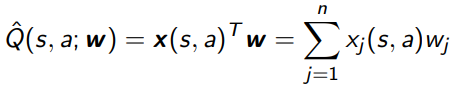
Functional representation

Just like before, you can represent the state-action with some feature vector and then let $Q$ be the inner product

Great table

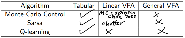
“chatter” means that SARSA will converge to a narrow window. For Monte Carlo on linear, this is active work.