• More readings

  

Moving towards IRL

You can’t infer a reward architecture by observation! Behaviors underspecify a reward stucture. But we can try and do a pretty good job. IRL is the process of inferring reward functions from expert demonstrations.

Why do IRL?

• imitation learning can lead to the same behaviors as the expert without any reasoning about action outcomes

• However, IRL allows us to infer the intentions of the demonstrator and perform the actions that leads to desired outcome (which may have never been shown).

So IRL allows you to essentially do better than demonstration.

As another reason: it can be hard to define a reward by hand in certain real-world situations. It can be helpful to automate the process from a set of expert demonstrations.

Older approaches

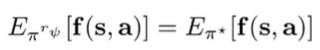
Feature matching

given a linear reward function $\psi^Tf(s,a)$, we assume that the features are really important to the reward. Therefore, given $r_\psi$, we want to find $\psi$ such that the expert policy and the learned $\pi^{r_\psi}$ optimal policy for $r_\psi$ have the same expected values for the features.

Intuitively: if we have good features and a good reward function, the learned policy will experience similar states and actions to the expert. However, there is a degree of ambiguity because a lot of different $\psi$ yields the same policy (if some states are just not visited, for example). This is important because feature mapping could just yield an arbitrary $\psi$ out of this ambiguous set.

Maximum margin principle

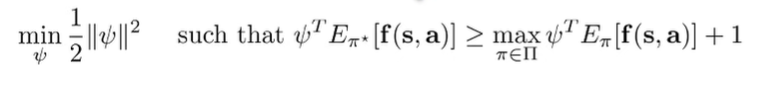
The Maximum Margin Principle is designed to resolve the ambiguity problem in feature matching. Instead of just trying to match features, the MMP wants to choose a $\psi$ that separates the optimal policy from all other policies as much as possible (sort of like a SVM)

The intuition is that you want to pick the $\psi$ that makes the expert look better than all the others. Of course, there is a problem: we may not be able to enforce the margin $m$ for all policies, because some policies are pretty similar to the expert.

We can use the SVM trick and formulate a different objective

and we can make an adaptable margin by changing the $1$ to a general distribution divergence measurement

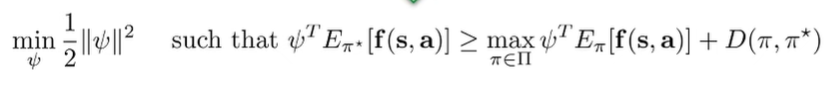
And this margin is more reasonable. However, this is still a heuristically-driven algorithm, and it’s not the best optimization problem either. Can we make an IRL algorithm from the ground-up?

IRL with Inference

The setup

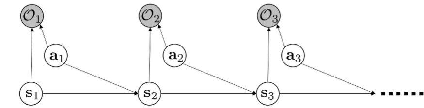
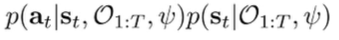
To help with our formulation, we go back to this PGM. We know that $P(O_t | s_t, a_t, \psi) = \exp(r_\psi(s_t, a_t))$. Previously, we tried to find the optimal policy. Now, we are interested in finding $r_\psi$.

Using Bayes rule, we can write the conditional distribution as proportional to $p(O_{1:T}, \tau)$

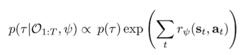
Moving towards optimization

We want to learn the optimality variable, i.e. we want to learn the conditional probability distribution $\exp(r_\psi(s_t, a_t))$. To do this, we propose a maximum likelihood objective

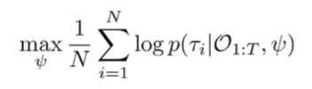
We remove that $p(\tau)$ term up front, as it doesn’t depend on $\psi$. If we plug in the exp-reward formula, we get

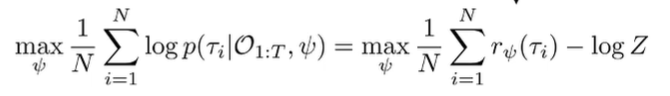
So this looks pretty good! It looks like we just need to optimize the reward, subject to the partition function. If we ignore the partition function, this reads “find the reward such that expert trajectories have high reward.” The partition function forces frugality in reward assignment.

The partition function

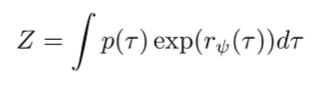
The partition function is generally not tractable because it’s an integral over trajectories

But what if we ignore this problem for a quick second? If we plug this into our objective, we get

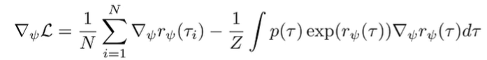
We can rewrite the second term as an expected value, because $p(\tau | O, \psi) = \frac{1}{Z}p(\tau)\exp(r_\psi(\tau))$. So we can rewrite it as

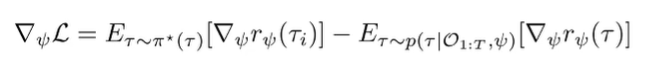
Now, this didn’t make the problem easier, per se, but it gave a nice interpretation. Intuitively, the gradient is just the difference between the rewards under the expert trajectory samples (given) and the soft optimal policy under your current reward $r_\psi$. We can use this interpretation to move forward.

Estimating the expectation

So we have a good interpretation, but how do we actually estimate this expectation? We can expand the trajectory as follows, using the linearity of expectation

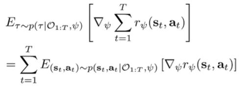
We can decompose the sampling distribution:

which is the state marginal and the policy. Now, recall that the policy is the ratio of backward messages (see control as inference) and the state marginal is the product of the forward and backward messages.

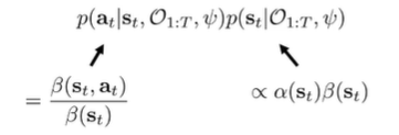
which means that

You can normalize it over a single state, not trajectory, so it is more tractable.

So, let $\mu_t(s_t, a_t) \propto \beta(s_t, a_t)\alpha(s_t)$. We can rewrite our expectation as

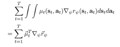
If we collapse the state-action visitation into a vector, we can express the expectation as an inner product.

If we have small and discrete spaces with known dynamics, we can compute this expectatin.

The MaxEnt IRL algorithm

We have just arrived at the classic maximum entropy inverse RL algorithm! At the heart of it, we are trying to compute this objective:

And in our workup above, we found a good way of doing this through the message passing

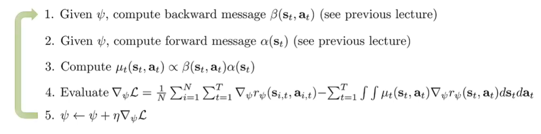
The Maxent IRL fits the observed points while maintaining entropy over unseen states.

High Dimension Approximations

Now, this MaxEnt IRL requires enumerating all state-action tuples, as well as solving for the soft optimal policy in the inner loop which requires knowledge of dynamics. So there are a lot to be desired.

Approach 1: Sampling

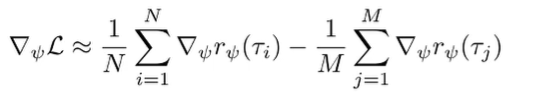
Here’s the objective again:

The first term you can sample from the expert. But what about the second expectation? Well, we can learn the policy $p(a_t | s_t, O, \psi)$ using any max-ent RL algorithm, and then use that policy to sample for the second expectation. This yields two summations

This is viable, but it does require the forward problem to convergence for every gradient step, and this is super slow.

Approach 2: Lazy Policy Optimization

What if we improve a continuous policy? In other words, we keep a policy between steps of the outer loop, and for each gradient step, we take a gradient step to improve this policy, before computing $\nabla_\psi \mathcal{L}$.

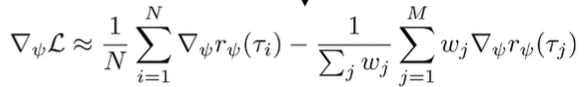
The problem is that this policy is now biased! It’s the wrong distribution. We can correct it through importance sampling

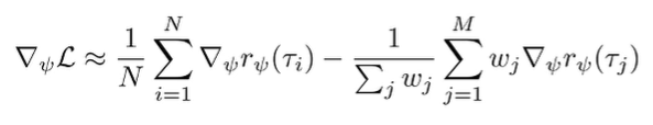
where we use the standard importance sampling format:

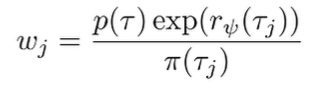
These importance weights can be calculated quite easily because most things cancel out and we get

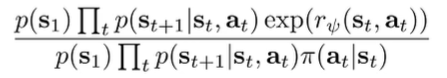
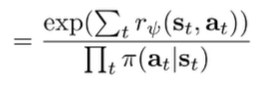
Everything here is calculatable! And here’s something interesting—when we update $r_\psi$, we bring ourselves closer to the target distribution, until hopefully the importance sampling weights become close to 1.

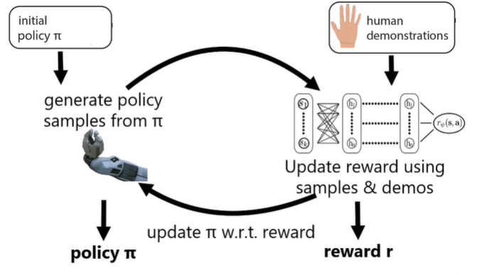
This is the premise of the guided cost learning algorithm (Finn et al.), which iteratively creates a good policy and reward

IRL and GANS (IRL as games)

We might notice that the structure of optimization looks like a game!

We are trying to make the expert demonstrations look good (first part), and the soft optimal policy look bad (second part). It’s an adversarial game! We are fitting a reward that is a discriminator, essentially.

IRL as a GAN

Recall that the GAN discriminator has an optimal target of

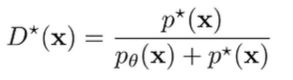
What about IRL? The optimal policy approaches $p(\tau)\frac{1}{Z}\exp(r(\tau))$. So let us consider this optimal discriminator that operates on $\tau$.

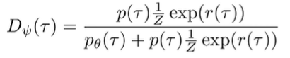
Note that implicitly, $p^*(\tau) = p(\tau | O_{1:T})$ and $p_\theta(\tau)$ has a simialr factorization (this step I’m actually not quite sure about). But if we cancel like terms, we get

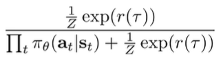
The discriminator will only output 0.5 if the policy probabilities are the same as exponential reward, which means that it has converged. The GAN objective is

Concretely…

• Discriminator tries to define $r$ and $Z$ to distinguish expert from all others (while adhering to the quotient form corresponding to optimal policy)
  • the special form means that we cotrain this reward function.

• Generator tries to make $\pi_\theta$ as indistinguishable WRT the current reward structure as possible

Can we use a regular discriminator?

If we just want to copy the expert policy, can we just use a regular discriminator?

Actually yes! It’s not an IRL because it doesn’t recover a reward, but it does recover expert policy in imitation learning. Just plug in a binary neural net classifier as $D$. You optimize against the discriminator in the generator step. For more, see GAIL (Ho & Ermon)

Good comparison of the two game methods

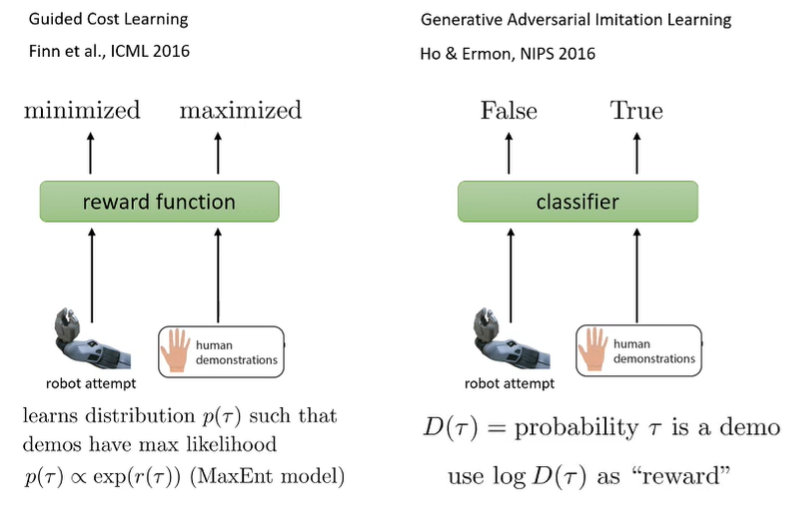
These are the same thing, but for the first one, you recover the reward as well.

Case study: Linear Feature Reward Inverse RL

Linear Approximations

Suppose that the true reward is just $r(s) = w^Tx(s)$, where $x$ is a feature vector and $w$ is the linear parameter. How do we learn $w$?

Well, using the definition of $V$, we can write this out:

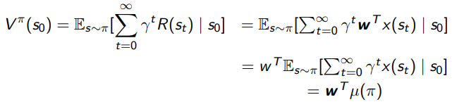
The $s\sim \pi$ is the expected trajectory (you can also read this as $\tau \sim P^\pi(\tau)$). So the inner infinite summation you can see as a discounted average of features through a trajectory, and we are taking the expectation across trajectories of this quantity. This is $\mu(\pi)$. We care about this, because it captures the places where the policy goes.

Feature Fitting

Here, we have a central observation: if we are within $\epsilon$ of the state distribution

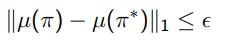
then for all $||w||\leq 1$, we have

which means that in this world, to get close to the demonstrating policy (assumed $V^*$), it is sufficient to just match feature distributions.

MaxEnt Reward Fitting

The MaxEnt algorithm tries to fit a $P(\tau)$, which is a distribution over trajectories. This distribution represents the policy, in this linear case. It relies on the Feature Fitting insight from the last section. Concretely, MaxEnt enforces these three objectives:

1. Maximum entropy of the trajectory distribution: $\max_P E_{\tau\sim P}[\log P(\tau)]$

2. Feature matching: $E_{\tau \sim P(\tau)}[\mu_\tau] = \mu(\pi^*)$. Here, the $\mu_\tau$ is the feature counts for a singular trajectory (corresponding to the $\sum_t^\infty \gamma^t x(s_t)$ in the setup, but we don’t use a discount because the trajectory is finite).

3. Distribution property of $P(\tau)$: $\sum P(\tau) = 1$.

It turns out that once you derive it through constrained optimization, you get the maximum entropy to be an exponential family distribution

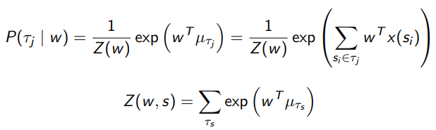
This is the policy that, given $w$ will give you the most reasonable policy that is also the most noisy. So you can imagine intuitively that for less important actions, it will do more random actions than a greedy policy.

This closed-form solution for the optimal policy is critical, because we are about to use this equation to learn this $w$.

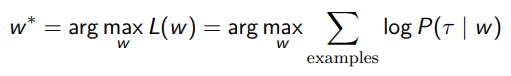
MaxEnt Learning W

The idea is simple: we want to make a $w$ to maximize the likelihood under the MaxEnt trajectory distribution

You can derive the gradient, which just becomes

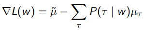
which is very similar to other sorts of regression, where we push a computed quantity to the real deal.

And in learning this $w$, you’ve learned the reward!