How do you collect demonstrations?

• kinesthetic teaching (use human hand to guide robot)

• remote controllers

• puppeteering (new approach), copy the leader

• watch videos of humans / animals
  • problem: no actions, different embodiment, different optimal strategies

Behavior Cloning

Basically you just minimize the policy to some collected expert dataset of states and actions. This is a regression problem.

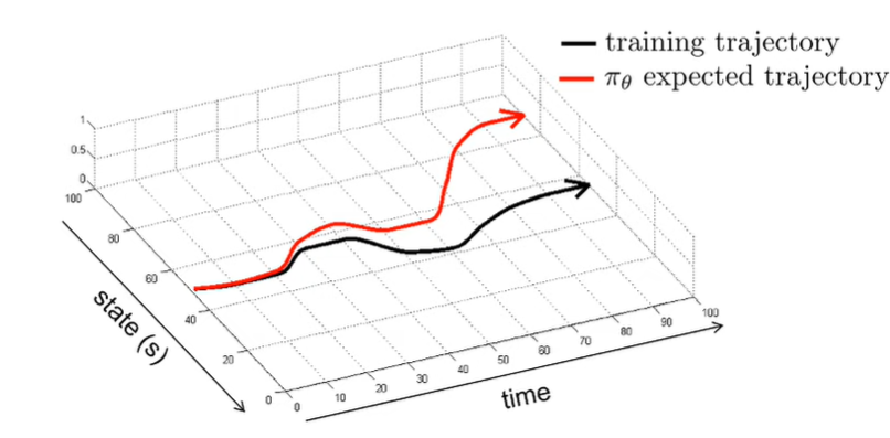
Unfortunately, this does not work very well. The main problem is that the expert only does good stuff, and they may not show how to correct mistakes. So the second that our model makes a mistake, it won’t know how to correct itself. This leads to compounding errors

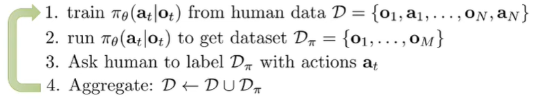
DaGGER Algorithm

A simple solution is to just show mistakes! If the agent learns how to correct the mistakes, then the agent won’t have compounding errors.

Another way of fixing this problem of distribution shift is to literally make the expert observation data distribution the same as the policy observation data. To do this, just let the agent run in the environment, but the expert provides the action labels. We call this DAgger, or Dataset Aggregation.

Primarily, this works, but for a human this is actually hard. Because the human doesn’t control the robot directly, it may overcompensate.

Other failures

There are three problems that can occur in the demonstration data

Non-markovian: In general, humans are non-markovian, which means that if we apply a markovian assumption, we essentially get conflicting data. Solution: add history

Causal confusion: What causes the behavior? What is concurrent with the behavior? This is the question of causality. Sometimes adding more information can make this causality problem worse. Solution: environment interactions and expert intervention (DaGGER)

Multimodal: given a certain situation, two very different actions can yield the same optimality. Solution: categorical distribution, or other complicated continuous distributions like GMM and VAE . Or, use autoregressive sampling

Expert knows more: there’s no model solution to this, because it’s a problem of data.

Imitation learning theory

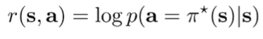
Cost function

Generally, when we optimize for imitation, we use log likelihood.

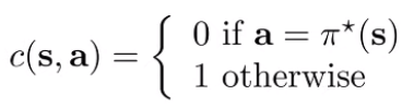
However, for theoretical analysis, we can also use an indicator function. We’ll see why this is useful in a second. (for distributions, you can think about sampling or taking argmax)

Bounding Naive BC: No Generalization

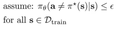
Let’s assume that we have converged well on the ERM objective up to some $\epsilon$, which means that

We want to see what happens when we run this policy in a pessimistic real-world situation, which we denote as the tightrope condition

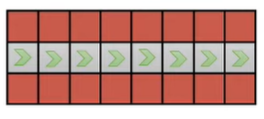
Under this condition, the policy must take the right action at every step. As soon as it takes the wrong step, we assume (pessimistically) that it gets itself into a bad state that it has never encountered before, meaning that it will make more mistakes until the end of episode ($T$ steps)

Immediately, we start to see a geometric series using the $\epsilon$ as the scaling factor. At any timestep $t$ with probabiltiy $\epsilon$, we make a mistake, and then we get stuck with mistakes for the rest ($T - t$ steps). With probability $1-\epsilon$ we don’t make a mistake and we get a cost of 0. This we can write recursively

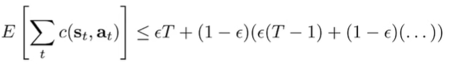
This is the error bound for every timestep $t$. We note that we never get anything beyond the $T$ term, so we say that the error is upper bounded by $O(\epsilon T)$ for each step. Therefore, the overall error bound is $O(\epsilon T^2)$.

Generalized analysis

In the previous derivation, we assumed the worst-case, where the policy does well on the training distribution and terribly anywhere else (hence the tightrope). Can we relax this condition? In other words, what happens if we introduce generalization?

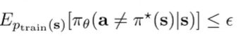
Concretely, instead of saying that the error is bounded for any $s\in D_{train}$ , we say taht the error is bounded for any $s\sim p_{train}(s)$. It’s actually sufficient for our derivation to say that the expected error is bounded by $\epsilon$, which is easier to obtain because it is our training ERM objective

💡

Note: DAgger pushes $p_{train} → p_\theta$, which means that we push towards the case where $\pi_\theta$ is always bounded by $\epsilon$, not just under the train distribution. In this case, we have

If $p_{train}\neq p_\theta$, then we can write the distribution $p_\theta$ as a convex combination of two distributions

This is analogous to a softer version of the tightrope. At timestep $t$, the chance that you’ve kept yourself in $p_{train}$ is $(1-\epsilon)^t$. We assume that if we do the wrong thing, we can never go back into the correct distribution (we get stuck in the mistake distribution)

In general we can’t say much about $p_{mistake}$. However, we can bound the total variational divergence in terms of our existing terms (TVD is just pointwise difference, literally just the meaning of an absolute value)

We are doing the total variational divergence because we can create a loose bound, which is 2 in discrete land.

We observe that $(1-\epsilon)^t \geq 1 - \epsilon t$, so we can use a looser bound $2\epsilon t$

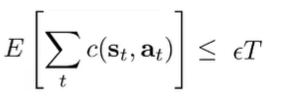
Finally, let’s compute the expectation of cost. We use the trick by adding $p_{train}$ and subtracting $p_{train}$ and putting absolute values around it

And we can plug in our previously derived bound for the thing inside the absolute values. We also know that the first term is bounded by $\epsilon$ by our setup. So, we get

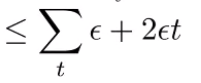
Which is bounded by $\epsilon T + 2\epsilon T^2$, which is still $O(\epsilon T^2)$. As such, even if we relax things with the generalization, we will get quadratic.