• Additional reading

  

  

  

The problem

State spaces can be very large, and you may never get to a good enough reward state to learn from it. What’s more, often local rewards are only weakly correlated to the final objective. How do we explore? This is actually a fundamental question of exploration vs exploitation. Do we keep learning in hopes of getting higher reward, or do we use what we have?

Count-based Exploration in MDPs

The basic idea

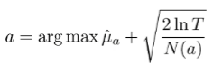
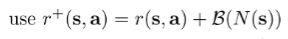
Previously, we had this formula for exploration in the bandit setting. Now, in the the MDP setting, we can use a similar idea. Let $N(s, a)$ be the number of times you’ve seen this state and done this action. Then, you can use an augmented reward

Hash counting

We can also just go back to normal counting, but we hash the state. You can use an autoencoder and it produces hash collisions when the states are similar.

Pseudocounts

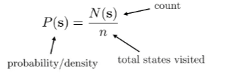
We can fit a density model $p_\theta(s)$ which tells us the likelihood of this state. Because it’s a model, it can interpolate.

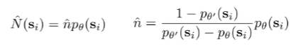
Now, we want to extract some notion of counts from a density model. As we see more states and fit $p_\theta$, the model changes. Can we extract a count that way?

To explore this option, we observe that for true count models, the following is true:

and after we see $s$, we get

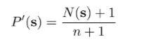
Which means that if we have both $P(s)$ and $P’(s)$, we have two equations and two variables. And therefore, we can solve for $\hat{n}$ and $\hat{N}(s)$.

• General Algorithm

  

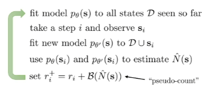
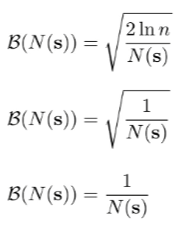
And then you can use this pseudocount in the UCB algorithm. There are some variants, but the big idea is that it decreases with $N(s)$. Here are some examples

and practically speaking, for $p_\theta(s)$, we need to generate a density score, and it doesn’t need to be normalized. Furthermore, we don’t need to sample from them. Therefore, we can consider using an energy model or something simpler.

Implicit density modeling

Instead of of explicitly representing the density function, we can also represent it implicitly through a classifier. The general idea is that we want a classifier to distinguish if something has been visited or not. The state is novel if it’s easy to distinguish from previously seen states, and it’s not novel if it’s hard to distinguish.

If we move briefly to theoretical analysis, if we have a classifier $D_s(s)$ that classifies a state $s$ against all past states, we can use the formula for the optimal classifier $1/(1+p_\theta(s))$ and solve for $p_\theta$

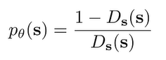
Now, this seems degenerate for a second, but remember that $s$ is also present in $D$, or at least a very similar version of $s$. So, $D_s(s)$ would not be $1$. The larger the count of $s$ in $D$, the lower $D_s(s)$ will be.

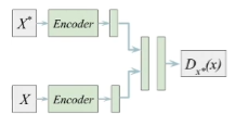
In real life, instead of training one classifier on each state, we can train one classifier that takes in two states and outputs the prediction.

Error-based counting

A novel example can yield higher errors when we try to fit the model to this state. Therefore, we can use the error as a novelty bonus!

• Algorithm

  

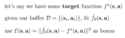
What do we use for this function? Well, we can use $f$ as the dynamics of the model $f(s, a) = s’$. We can also use $f^* = f_\phi$, where $\phi$ is a random vector. As long as we have something that varies non-trivially with the states and actions, we can get a notion of error. (The random vector case is good because you don’t have to refit a model every time.)

Thompson sampling in MDPs

Thompson sampling in Bandits is sampling parameters and then using greedy selection on these parameter samples. The analog in MDPs is to sample Q functions and act according to that Q function for an episode. We can accomplish this by using a Q function ensemble and select heads at random.

Why does this work?

So Epsilon-greedy is random WRT actions, which basically result in random vibrations. But if we sample Q functions, we essentially sample different life philosophies. It’s an abstraction on randomness

in general, it doesn’t work as well as count-based, but it also doesn’t require any hyperparameter tuning and it’s pretty intuitive. We train this model from bootstrapped data.

Information gain in deep RL

We want to select in an action that gives us the most information about some hidden variable, $z$. But what information do we care about? Reward? But that’s sparse.

But what about state density? If we want to gain information about state density, you’ll do novel things.

What about dynamics? Gaining information about the dynamics means that we are leaning things about the MDP.

State density and dynamics are good, although they are mostly intractable. We need to make some sort of approximations.

Approximating the information gain

We can try prediction gain, which is just

We can also use a stronger method by modeling a hidden variable $z$ and optimizing for

This objective is explored in VIME

VIME

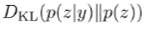
In our case, $z = \theta$, and our observation is a transition $(s_t, a_t, s_{t+1})$. So, our objective is

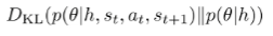
where $h$ is the history of prior transitions. Of course, this objective is not tractable because you need to estimate $p(\theta | …)$. We use variational inference to estimate an approximate posterior $q(\theta | \phi) \approx p(\theta | h)$ and this allows you to optimize the variational lower bound to

This is the same objective as above because $p(h | \theta)p(\theta) = p(h, \theta) = p(\theta | h)p(h)$, but because $p(h)$ doesn’t involve $\theta$, we can remove it.

We can express $q(\theta | \phi)$ as a product of independent gaussians (so a Bayesian neural network), and the $\phi$ represents the means and variances of the gaussians.

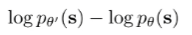
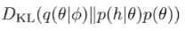
During test-time, we can fit the model to get $\phi$ but also $\phi’$, which is the model after we get the new transition. Then, we compute

So essentially, you try updating the network and we add a bonus to the amount that the parameters change, which is the same as information gain.

Other ways of using information gain

• use model error or model gradient, etc