Reframing Control as Inference

The big idea is looking at the big RL objective as an inference problem as an attempt of better explaining natural behavior. To begin, we need to talk about a special model.

Human and Animal Behavior

Our objective is to explain elements of human and animal behavior through models. But how do our existing models fall short?

• When we hit a goal, some of the intermediate states matter less (so we get a state distribution that get wider in the middle)

• Humans & animals are not completely optimal, but they happen in places that matter less for the task. Why is this the case?

If we believe that natural behaviors are stochastic, we need to use this in our analysis.

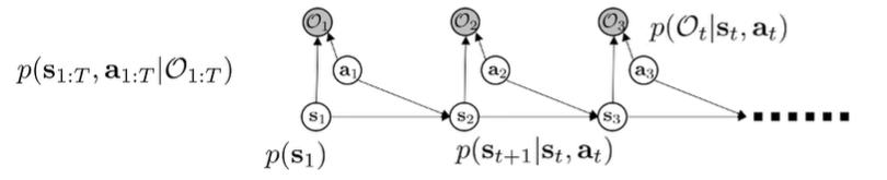
The Model

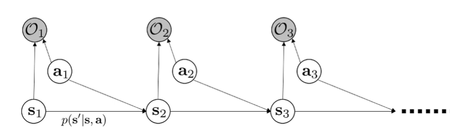
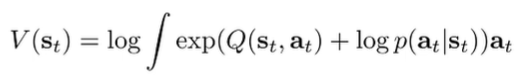
We can formulate optimal control as a PGM. Normal MDP PGMs just contain state-action influences, but in this case, we also add an observed optimality variable. We want to observe that $O_{1:T} = 1$ for all $t$, because we are trying to do well. This is a little weird, but bear with me.

• Optimality $O$ is a binary RV (a design choice)

• We choose to define $p(O_t | s_t, a_t) = \exp(r(s_t, a_t))$. Now, this is somewhat arbitrary, but it leads to a nice formulation.
  • we need rewards to all be negative, but this is a minor technicality

• We have multiple inferences of interest; see below.

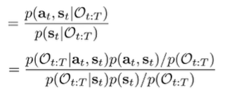
Moving towards the inference

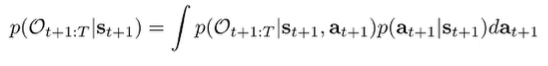
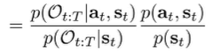
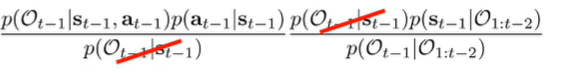
We can start by using Bayes law and we have a formulation for the numerator if we factor it as $p(O_{1:T} | \tau)p(\tau)$:

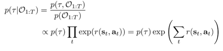
So this suggests that we weight the probability of trajectories by the rewards of the trajectory. But the interesting part is that the suboptimal trajectories are not destroyed; it just has lower probability of existing.

This also accounts for multimodality! The same rewards have the same probability. This allows us to model suboptimal behavior, which is harder for hard optimality algorithms.

This is important for inverse RL, because it is a good model for behavior.

Inference through message passing

There are three inference we are interested in

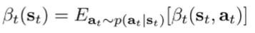
1. Backward message: $\beta_t(s_t, a_t) = p(O_{t:T} | s_t, a_t)$. Basically: probability of being optimal from now until the end of time, given a certain state and action. This is the backwards message because it’s easiest to start from the end of the MDP graph and move back

2. From this backward message, we can recover the policy $p(a_t | s_t, O_{1:T})$.

3. Forward message: $\alpha_t(s_t) = p(s_t | O_{1 : t-1})$. Basically, given that we are acting optimally so far, how likely is this state to happen? This is the forward message because it’s easiest to start from the beginning of the MDP and move forward

Let’s look at each of these inferences closely

Backward Messages: The Setup (1)

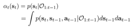
Here’s the big idea: if we know $p(O_{t:T}, s_{t+1} | s_t, a_t)$, then we can marginalize out $s_{t+1}$ to get $p(O_{t:T} | s_t, a_t) = \beta_t(s_t, a_t)$. But how do we get $p(O_{t:T}, s_{t+1} | s_t, a_t)$?

By the graph structure, we know that $O_{t+1:T}$ is independent of all optimalities in the past when conditioned on $s_{t+1}$. This gives a convenient factorization of

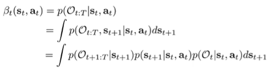
We know the dynamics from the model and $p(O_t | s_t, a_t) \propto \exp(r(s_t, a_t))$. The first component $p(O_{t+1 : T} | s_{t+1})$ is not known, but we can make it recursive by writing it like this:

and of course, this is just the integration of the future backward message $\beta_{t+1}(s_{t+1}, a_{t+1})$ with the action prior $p(a | s)$. (this is not the policy, because we are not conditioning on optimality. We can often just represent this with a uniform distribution.

So we’ve just created a recursive construction of the backward message. We can rewrite the integral construction as an expectation

where we define $\beta_t(s_t) = p(O_{t+1:T} | s_{t+1})$. This too can be written as an expectation, if we consult the integral.

The computation of the backward messages are simple: just follow these two expectations! At the end, you know what $p(O_T | s_T, a_T)$ is (by our construction), and so you are done.

Backward Messages and V, Q Functions

Now let’s compare this algorithm to standard RL approaches. Let’s start by suggestively defining these variables

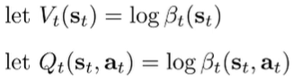
If we write $V$ definition using the beta definitions in log space, then under the assumption that the action prior $p(a_t | s_t)$ is uniform, we get

This is a log-sum-exp, which is a soft maximum! So it’s a soft version of $V(s_t) = \max Q(s_t, a_t)$.

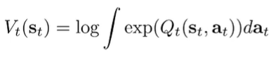
Now, if we write that Q definition in log space, we get

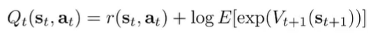
where $E$ is the expectation over transitions. And this looks a lot like the bellman backup! The difference is that this second term is a soft maximization as well. So this is a little suspect, because we are not taking the softmax across actions. It is the softmax across states. And this means that we have a bias of assuming lucky situations.

This problem arises from asking the bad question: When we ask $p(a | s, O)$, we don’t distinguish if we get good because of good actions or if we get lucky! We will resolve this problem in our variational setup.

Why we don’t care about action prior for Backwards Messages

If we have a non-uniform action prior, the value function becomes

But if we rewrite the Q function as the follows:

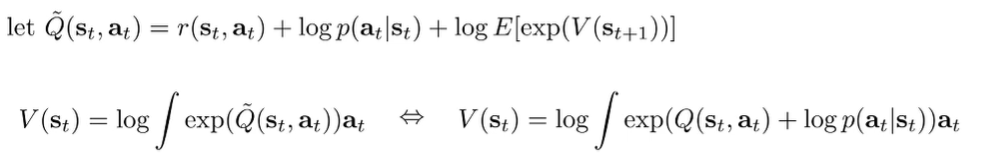
Which means that the relationship between Q and V is not changed. Rather, you’re just operating with an added $\log p(a_t | s_t)$ to the reward. This is why we don’t really care about the action prior.

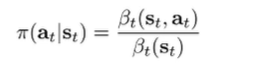
Policy computation (2)

Note how $O_{1:t-1}$ is D-separated by $s_t$ from $O_{t:T}$. Therefore, the policy can be simplified into

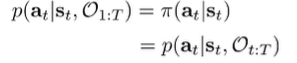
which is why we can recover the policy using backward messages only. We want to get this in the form of the backward messages. So let’s begin this inference by applying Bayes rule twice.

We cancel like terms, and we get

The second fraction is $p(a_t | s_t)$ which is the uniform action prior. But the first fraction is just the ratio of backward messages!

And this has as really nice interpretation. In log space, we previously established Q and V in relation to the messages. And so the ratio can be expressed as

So the likelihood of an action is related to the advantage of that action. The higher it is, the more likely you are to take that action. It is “soft” learning!

We can add a temperature to control the “softness”

Forward messages (3)

We care about the forward messages because of some later analysis. We continue in a simialr manner by adding and marginalizing $s_{t-1}, a_{t-1}$

We factorize with future inference in mind

The first term is just the transition probability ($O_{1:t-1}$ is d-separate from $s_t$ given $s_{t-1}$ and $a_{t-1}$), But what about the second and third terms? We can use bayes rule again.

For the first fraction, we flip $O$ and $a$. For the second, we flip $O_{t-1}$ and $s_{t-1}$ (so not the whole optimality chain)

We can cancel the term $p(O_{t-1} | s_{t-1})$ from both sides which gets us this:

The $p(O_{t-1} | s_{t-1}, a_{t-1})$ is defined in terms of reward, the $p(a | s)$ is action prior, and the $p(s_{t-1} | O_{1 : t-2})$ is the recursive definition. The $P(O_{t-1} | O_{1:t-1})$ is a normalization constant.

The base case we have just $\alpha_0(s_0) = p(s_0)$, which is given.

Deriving state marginals

What if we wanted $p(s_t | O_{1:T})$? This is the state marginal, which is the state distribution given that you’re acting optimally. Well, with the forward and backward messages, we can do exactly this! We use Bayes law and factorization

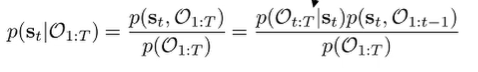
The first term on the numerator is just $p(s_t | O_{1:t-1}) = \beta(s_t)$. The second term can be written as

which is $\alpha(s_t)$ a normalization term. So, we can write the marginal as

But what is the intuition behind this expression? Well, we can imagine the backward message as a distribution of viable states from which you can reach the goal. This widens as you move backwards.

You can imagine the forward message as the distribution of viable states an optimal agent can reach if starting from a certain start point. The state marginals is the intersection of the two cones, because 1) you’re starting from the beginning and 2) you’re reaching the goal

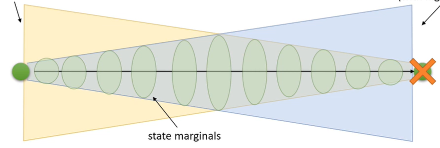
The intersection of two distribution show a widening and narrowing as we go from start to end. This is consistent with behavioral results, which show higher entropy in the middle of a trajectory.

Control as variational inference

If the dynamics are not known, or if things are complex, we can’t do exact inference. So let’s talk about how we can use variational inference.

The optimism problem (motivating Variational Inference)

This is going to be dominated by the luckiest state transition. Example: if you are buying a lottery ticket, the Q value of getting a lottery ticket will be very large, because we are taking a soft maximum. It’s falsely optimistic!

But it’s not a mathematical problem. It’s a philosphical one. When you wnat $p(a_t | s_t, O_{1:T})$, you’re asking “given that you obtained a high reward (O_1:T), what is the action probability”. If we asked a lottery ticket winner this question, they would say “I bought a lottery ticket”. It is a correct answer to a bad question!

Mathematically, it is because

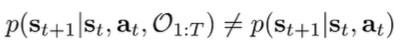
Optimality is D-separate given past states, but future optimality can influence present actions. This makes sense. It’s like peeking into the future allows you to influence the present chance.

We can resolve this problem by casting the inference as a constrained problem that keeps the existing dynamics. More on this below.

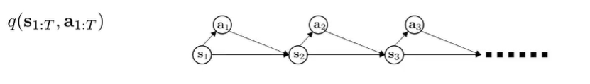
The variational setup

We want to find a distribution $q(\tau)$ that is close to $p(\tau | O_{1:T})$ while having the original dynamics $p(s’| s, a)$. Let’s start with modeling $q$ as a factored distribution. Note that we bake in the dynamics into the distribution and we only modify the $q(a | s)$. This prevents the optimism bias we talked about in the previous sections

Graphically, we are trying to fit a slightly different model to the original $p(\tau | O_{1:T})$.

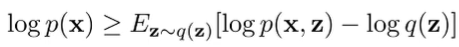
The lower bound

The standard ELBO is in the following form:

and if we sub in $q(z) = q(\tau)$ and $p(x, z) = p(\tau, O_{1:T})$, we get

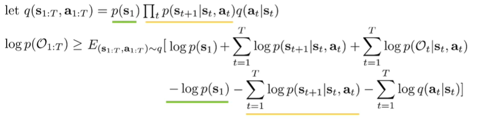
And the transition and initial distributions cancel out, which gets us

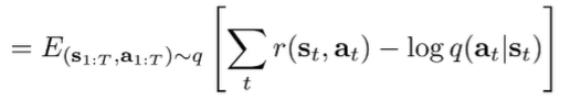
So this tells us that if we want to increase the probability of $p(O_{1:T})$, we need to increase the reward while maximizing entropy of the function (that’s the log term). Note that $q$ is a distribution over $\tau$, so this is the original RL objective with an entropy term.

Optimizing the lower bound

The big idea is to solve for Q and V through optimizing the lower bound. Let’s look at the last timestep first, which only has one step to worry about. Let’s derive this base case.

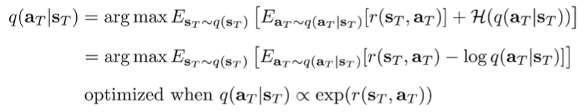
Now, if we write out the actual distribution, we get a nice result:

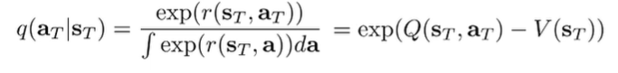
^^this is true because the value function is the log-int-exp of the Q function in our soft setup. The Q function is just the summation of rewards

And we can plug this into the original objective to get

Now, let’s move to the recursive case, where the objective becomes

And if we substitute the regular bellman backup into this equation, we get

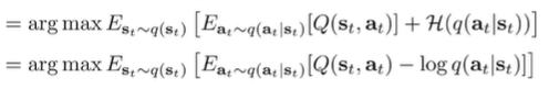
Because it is in this particular form, we know again that it is optimized when $q(a_t | s_t) \propto \exp(Q(s_t, a_t))$.

This is recursive because each step relies on $V_{t+1}$ which is defined in terms of $q(a_{t+1} | s_{t+1})$and it allows us to compute Q and V in the process.

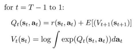
and we’ve just derived value iteration again, except that we take $V$ as the soft maximum of $Q$. Note how this is different from the original backward message: We are no longer taking the best possible state in the $Q$ update. We are only optimizing over actions. This prevents over-optimism, and it’s all because we constrained our model to follow dynamics!

Algorithms derived from this theory

Soft Q learning

The standard Q learning is as follows:

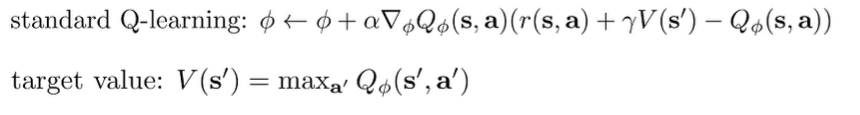
we can “soften” this by changing the target value to be a soft maximum:

and the policy is as follows

Soft Policy Gradient (Entropy-Regularized Policy Gradient)

You just need to maximize policy entropy!

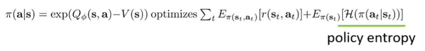
Intuitively, we want to bring the policy $\pi(a | s)$ as close to the soft optimality of $Q$ as possible, which is $\exp(Q(s,a))$. We minimize the KL divergence, and this KL divergence has the following setup

We call this an “entropy-regularized policy gradient”, and it helps with exploration.

If we write the gradient out, we get

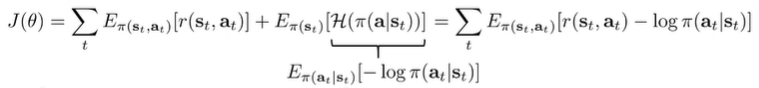
And the gradient becomes (after some algebra calculation).

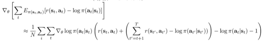
And it turns out that this is just the normal policy gradient with an entropy component to the reward. So if you want maximum entropy policy gradient, just subtract $\log \pi(a|s)$ from the reward!

Literature review

Traditional RL algorithms will commit to one arm of a multimodal problem. With soft optimality, there is no hard “commit”, which means that it can be fine-tuned better.

Some additional readings

Reinforcement Learning with Deep Energy-Based Policies Haarnoja, Tang, Abbeel