Multiarmed Bandits

A multi-armed bandit is a stateless tuple $(A, R)$ where you take some action out of $n$ possible choices. This corresponds to sampling $p(r | a)$. As a simple example, you can think of each reward distribution as being a separate distribtuion, and the action $a$ selects that distribution. The term bandit comes from slot machines.

If you knew the expected reward for every $p(r | a)$, the problem becomes trivial. You just keep on exploiting the one with the highest expectation. But the key is that you don’t. The goal of the bandit is to maximize the cumulative reward through your trials. So you can imagine that this is a study in learning quickly the parameters of $p(r| a)$.

Regret 🐧

We define an action-value function as $Q(a) = E[r | a]$. Intuitively, this is the average reward you get for action $a$. If the true $Q$ were known, control would be trivial. We define the optimal value $V^* = Q(a^*) = \max Q(a)$.

The regret is just the opportunity loss for one step:

And the total regret is the total opportunity loss:

We can rewrite the total regret in terms of gaps, which we define as $\Delta_i = V^* - Q(a_i)$. With this, we have

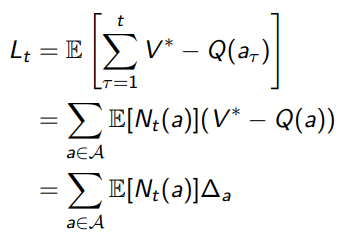
Where $N_t$ is a counting variable. So you can sort of understand that a good learning algorithm keeps small counts for large gaps, where the actions are very sub-optimal.

What are we looking for?

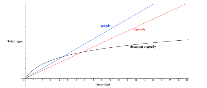
Bad learning algorithms are linear in regret, with respect to time step. Intuitively, it means that there is always a performance difference between the algorithm’s actions and the optimal action, on average.

A good learning algorithm will close that gap, leading to sub-linear (think integral and area between the learning and expert reward curves) or logarithmic regret. This is better!

Regret Lower Bound

Given an ideal learning algorithm, is there a best possible performance? As it turns out, we can describe it in terms of $\Delta_a$ and the KL divergence between the different reward distributions for each action.

Intuitively, the more similar the distributions or the more similar the expected values, the longer it takes to learn.

Greedy Algorithm

As you explore, you keep track of your $Q(a)$. In greedy exploration, every action is just the $a$ that yields the maximum of your current $Q(a)$. You recompute the $Q(a)$ every time using your sampled reward.

What’s the problem?

Well, a greedy approach can lock onto a suboptimal action forever. Suppose that you got really unlucky with an optimal distribution, and you got a very low number. Then, you might lock onto a mediocre distribution whose mean reward is higher than this low number from the optimal distribution.

In this case, you will never explore the optimal distribution again. And in terms of regret, if you land on a suboptimal state, then you will incur linear regret.

Epsilon Greedy 💻

The epsilon greedy incurs some exploration. With probability $1-\epsilon$ use the greedy policy. Otherwise, select an action at random. While this can prevent suboptimality, it is also true that we will be making a suboptimal decision $\epsilon$ fraction of the time.

Therefore, if you have a constant $\epsilon$, the policy will have linear regret (on average, there is a performance gap). While we may suffer no longer from the problems of greedy selection, we add a guaranteed suboptimality.

However, the problem here is easily solved by adding a decay factor to the epsilon, and we get the suboptimal regret

Optimism Under Uncertainty

This approach is actually pretty intuitive: assume that stuff you haven’t explored is worth trying. Why? Well, you either land on a better place, or you learn something (”you either win, or you learn”)

Upper Confidence Bounds

To do this sort of learning, you need to estimate an upper confidence bound $U_t(a)$ for every action. The goal is that $Q(a) \leq U_t(a)$ with a high probability. Then, you select the action by maximizing this bound.

UCB1 (Upper Confidence Bound) algorithm 💻

• Hoeffding’s inequlaity

  ☝

  this section is repeated in Math Theory

  If you have $X_1, … , X_n$ IID (same distribution), then we have $E[X] = E[X_1] = … = E[X_n]$. Now, we want to estimate this quantity through these $n$ samples. A reasonabble start is to consider $\hat{X} = \frac{1}{n}\sum X_n$

  With this setup, we have

  $$P(E[X] > \hat{X} + \epsilon ) \leq \exp(-2n\epsilon^2)$$

  as well as

  $$P(|E[X] - \hat{X}| > \epsilon) \leq 2\exp(-2n\epsilon^2)$$

  (this entails naturally because the $u$ is squared on the right hand side)

  Intuitively, the more samples and the smaller the margin $u$, the lower the probability of violation.

From the Hoeffding’s inequality, let $\delta$ be the probabilty of violation. Therefore, we have

and you can solve this algebraically to become

and this yields the UCB bound:

This has a slightly different form due to some constants shifting around, but essentially you’re epsilon-bounding the true Q value with probability $1-\delta$ of being correct. And by adding this bound, you’re saying that this $UCB(a)$ has probability $1-\delta$ of being larger than the true value (because this estimate $Q(a)$ is subject to Hoeffding’s inequality, and adding that part of the epsilon ball boosts it past the true value.

The tl;dr is that the UCB is just a confidence interval around the Q value.

Choosing $\delta$

If there are a fixed number of time steps $T$, then you can let the inner term be $T/\delta$, or $t/\delta$ where $t$ is the actual timestep. We call this union bounding.

The reason is that you will be testing the bounds $T$ times, and remember the union bound:

Remember that the inner term is the reciprocal of the bound failure probability, and $T * \frac{\delta}{T} = \delta$. So this additional $T$ or $t$ term just make the overall failure probability bounded by $\delta$.

Properties of UCB

1) Shifting confidence intervals, 2) deterministic w/o extra data

You can imagine UCB as creating a confidence interval around the current $Q(a)$. However, this confidence interval may get larger or smaller as we progress. Consider the infinte horizon case where

If this action we discover to be sub-optimal and stop doing $a$, then the numerator will grow as $t$ increases. Eventually, the boost will be large enough for us to check again. It’s essentially making sure that we aren’t prematurely rejecting a hypothesis. So that’s why the confidence bounds can grow and shrink.

And its also worth noting that without extra data, the UCB algorithm is deterministic. This could be a problem with delayed rewards.

Regret bound of UCB

If we follow the UCB, we get the following guarantee:

$$P\left(|Q(a) - \hat{Q}_t(a)| \geq \sqrt{\frac{C\log \frac{1}{\delta}}{N_t(a)}}\right)< \delta$$

And we can relate this to $Q(a^*)$. First, we assume 1) that the bound has not failed us, i.e. $Q - \hat{Q} \leq \sqrt{C \log(1/\delta)/N(a)}$ and 2) that we have chosen this sub-optimal action $a \neq a^*$

From 1), we have

From 2), we have

and if we combine them we get

which yields

This indicates that if the original bound hasn’t failed, then we have

$$N_t(a)\leq \frac{4C\log\frac{T}{\delta}}{\Delta_a^2}$$

which gives a count on all the arms.

☝

Here we replace $1/\delta$ with $T/\delta$ because we are constraining the whole horizon to within the probabiliyt (see discussion on $\delta$ above). You can also replace it with $t/\delta$ for infinite horizons.

We can use this count to find the number of times we hit sub-optimal arms and weigh it by the Q delta, which is the definition of regret.

$$\sum_a\Delta_a E[N_T(a)] \leq \sum_a C' \frac{\log T}{\Delta_a}$$

which is sub-linear.

Is Pessimism ok?

Actually, Pessimism isn’t ok. Consider the following example

In this case, you will always pick the suboptimal arm (left), which yields linear regret.

Is UCB always the best option?

The answer is no. It is sub-linear asymptotically, but for one-shot or few-shot deployments, UCB can be very bad. Consider this example:

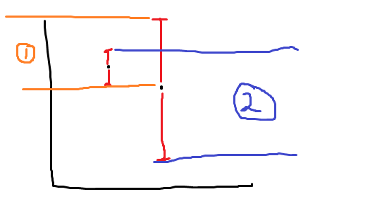
In UCB, we’d pick the second arm. However, the maximum regret (assumping PAC condition) is larger (blue) than if you were to pick the first arm. So, if you are to give your best few-shot estimate, UCB may have a worse worst-case situation. In this case, you may choose to go by means instead.

Bayesian Bandits

Previously, we’ve looked at ways of estimating the value of each action using $Q$. We can also take a bayesian approach, where we model $p(r | a)$

Concretely, we would perform Bayes rule

or if we have access to the conjugate distribution, you can use that too. In the notation above E(which we will continue to use), $\phi_i$ is the parameter for the reward of the $i$th arm, $r_i$ is one observed reward after pulling arm $i$. You’re performing a Bayesian update.

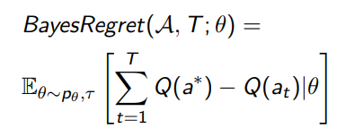
Bayesian regret

We just have to add another expectation over parameters, which define the $R$ which define the $Q$:

Probability Matching

We define probability matching as selecting an action according to the probability that it is the optimal action. Or, more formally,

This factors in uncertainty: if you don’t know, then the probability of optimality can’t be too small.

Thompson Sampling 💻

The basic idea is this: keep reward distributions $p(\phi_i)$ on hand. For each arm, in every step, sample a reward distribution and compute the Q value for it (most of the time, it is just the sufficient statistic $\phi_i$ that you sampled). Then, take the action that maximizes this current Q, and update the explored posterior using Bayes rule or conjugate distributions.

• Algorithm box

  

• Example for Bernoulli and Gaussian

  For Bernoulli, just add 1 to $\alpha$ every time you observe a positive result using the given sample of parameters. Add one to $\beta$ every time you observe a negative result

  For gaussian, just update the mean like you normally would.

Wildly enough, Thompson sampling is probability matching! This is not immediately obvious, but you can rewrite the probability matching equation as

where Q is derived from R. And this is just the Thompson sampling definition.

Information Gain

We can also use something more sophisticated as an exploration strategy. If we had an estimate of $H(p(\phi))$ (the distribution of all parameters) then we’d want to take some action such that $H(p(\phi) | r_a)$ decreases the most (i.e. you learn the most from this action). We write this as

And smilar to previous approaches, we have the expected suboptimality of an action, $\Delta(a) = E[r(a^*) - r(a)]$. We pick an action by balancing information gain with suboptimality according to

Which do you use? 🔨

• Thompson sampling is dynamic even without new data, which can be useful if you’ve got parallel operations. In contrast, optimism based approaches will not change if you don’t add more data

• Thompson sampling needs a reasonable prior, so this is something you need to fine-tune. In contrast, optimism approaches don’t need any sort of tuned prior.

• Thompson doesn’t perform obviously better or worse than UCB

• Information gain works well, although it may be difficult to estimate the entropies of the parameter distributions

Probably Approximately Correct 🐧

So in regret, we considered essentially the area between the optimal value and the learning value. That was one way of analyzing the learning process. Unfortunately, Regret can’t separate a model that makes a few large mistakes, or lots of little mistakes.

Here, we present another metric: probably approximately correct (PAC).

If a model is PAC, then it will choose an $\epsilon$-optimal action with probabiltiy at least $1-\delta$ on all but a polynomial number of steps (the burn-in time).

• $\epsilon$ optimal means that $Q(a) \geq Q(a^*) - \epsilon$

• polynomial number of steps means that convergence takes only polynomial time

Note that unlike Regret, PAC doesn’t care about precise optimality.

Contextual Bandits (brief) 🐧

A contextual bandit takes in a state, in addition to an action. So the reward distribution is $p(r | s, a)$. This is closer to the MDP, because your $s$ can evolve through time.

Modeling

We typically model a contextual bandit through a linear function of input features: $r = \theta^T\phi(s, a) + \epsilon$ where $\epsilon$ is a noise vector.

We do this because it allows for different states and actions to share information. And so instead of updating just a table of rewards, you’ll be updating $\theta$.