What’s wrong with policy gradient?

Well, a few things. First, the sample efficiency is poor because of the Monte Carlo approach.

Second, the distance in parameter space is not the same as policy space! Depending on parameterization, a small nudge in one parameter can yield a huge change in the policy’s overall behavior, because one parameter can impact a lot of things.

Off-Policy Policy gradients

Normally, policy gradients are on-policy because we need to take the expectation through $p_\theta(\tau)$. Can we make policy gradient off-policy?

Importance Sampling for Policy Gradients 💻

We can address the first problem of data efficiency through importance sampling. Why don’t we collect stuff through an old policy and use importance sampling to compute the policy gradient?

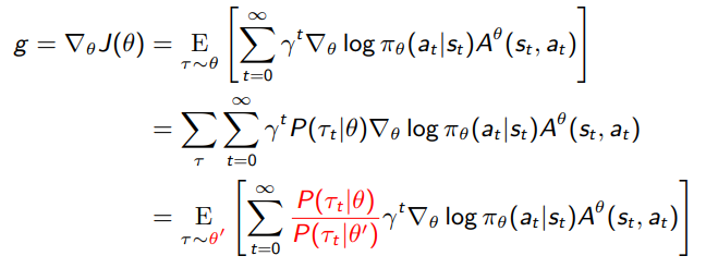
The ratio of trajectory distributions simplifies a lot

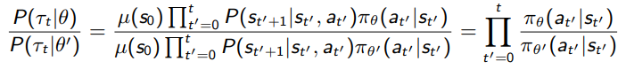
But you see a pretty big problem here. We don’t want the importance sampling ratio to be too big, or else bad things happen (unequal weighting, etc). But with a bunch of products, things can become very large or very small very quickly.

First-order approximation of importance sampling

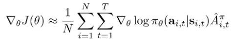
Can we rewrite our importance sampling and make an approximation? Well, here’s the insight: we can take the monte carlo across trajectories, or we can slice the trajectories into state-action marginals at every timestep. This is just a different way of interpreting the same sample. If we interpret it this way, we get this gradient

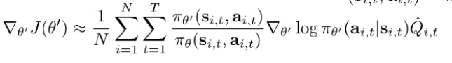
This isn’t very useful because we can’t actually compute these marginals. However, this allows us to do a little trick using chain rule:

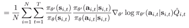
And we can make the (untrue) assumption that the state marginals are the same. In this case, we can just ignore everything that came before and taking the ratio of action probabilities! This means that you can remove the product of importance weights and only take one ratio.

Now, when will ignoring the state action marginal differences be ok? We’ll expand on this in the sections below. The tl;dr is that we need to change $\pi$ slowly.

Conditioned Optimization

Here’s a pretty big challenge: remember that policy-space is different than parameter space. Even if we use a small learning rate, we might just step too quickly at one point in the policy and yield performance collapse.

This is not a problem limited to the policy gradients; this is a general optimization problem. Traditionally, when we step in gradient descent, we optimize the following objective:

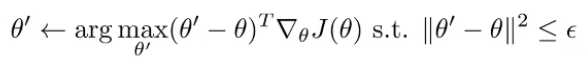
But theta space isn’t the same as policy space; this objective is sensitive the parameterization. Can we make things agnostic to parameterization? This forms the new objective

But how do we do this? The KL is hard to optimize directly, but the second order Taylor expansion yields

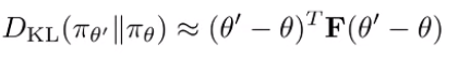
where F is the fisher information matrix

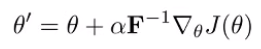
We approximate F using samples from $\pi$. Concretely, if you write down the lagrangian and solve, you get the new update

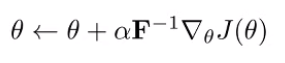
So this is just the transformed gradient descent.

Intuitively, recall that quadratic matrices will determine the shape of a quadratic form. The identity matrix has symmetry WRT the parameters, which corresponds to the L2 norm. With the Fisher matrix, we squish the quadratic form and make it selectively sensitive to certain parameters. Which parameters? Well, the parameters that cause the KL divergence to go up the most! And so we should be the most careful around optimizing these parameters!

Different flavors of natural policy gradient

Many algorithms use this trick. Natural gradients will pick an $\alpha$ . TRPO will select $\epsilon$ and derives $\alpha$ while solving $F^{-1}\nabla_\theta J(\theta)$. We will talk about this more in the next few sections. We will also show that if we do this correctly, we’ll get monotonic guarentees.

Policy Gradient Monotonicity (trust regions)

In an ideal situation, policy gradient is a weighted regression, using weights from the advantage function.

You alternate between estimating the advantage of the current policy $\pi$ and using this estimate to improve the policy. This is similar to value iteration and other forms of value-based methods!

Of course, this raises the question: why does this actually work? In value iteration and policy iteration, we showed things like contractions and monotonicity in tabular environments. In the following sections, we will derive a set of rules that will ensure monotonic improvements for policy gradients.

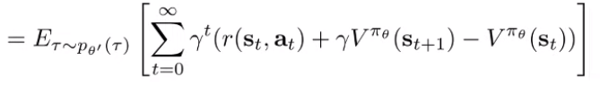
Performance Difference Lemma 🚀

Let’s start by considering $J(\theta’) - J(\theta)$. We claim that

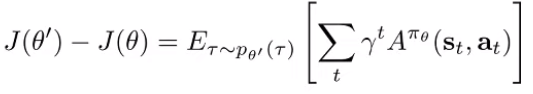
We care about this value because we want to eventually derive some rules that show that this quantity is non-negative.

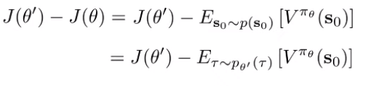
• Proof

  Replace J(theta) with an expectation. And note that we replace $p(s_0)$ with $p_{\theta’}(\tau)$ because the starting distributions are the same.

  

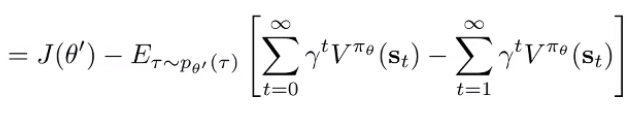
  And you use a trick: take the difference of infinite sums (look at this for a second and it should make sense)

  

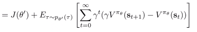
  You can rearrange the terms in the sums to get a telescoping summation

  

  Next, rewrite $J(\theta’)$ in terms of an expectation

  

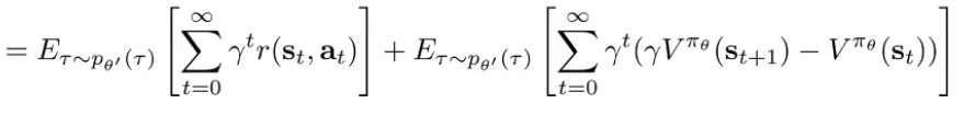
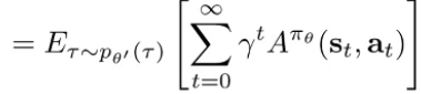
  Which should allow you to combine the terms and get you the advantage function

  

  

• Alternate proof (definition of V as expected reward, add and subtract a term. Note that we swap the role of $\pi, \pi’$ and we also use $V$ instead of $J$.

  We can also write this in terms of the discounted state distribution $d^\pi(s)$

  

  

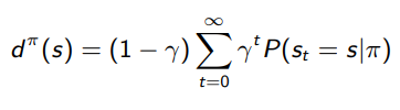
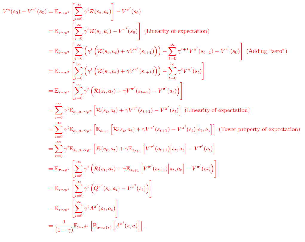
  For the last step, see the proven identity in previous notes.

The critical approximation

We can write out the expectation over advantages in terms of the state action marginals, which gets us

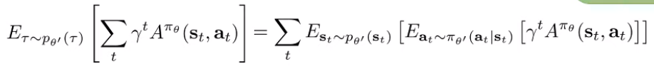
And we can rewrite the inner expectation in terms of $\pi_\theta$ through importance sampling

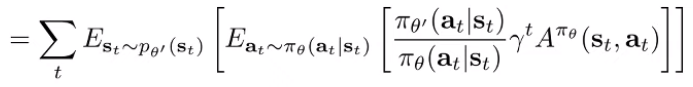
Now, we are left with one tiny problem. We can sample from $\pi_\theta$, but we can’t sample from $p_{\theta’}$ because it’s something we don’t have yet. But can we assume that the state distribution of $p_{\theta’}$ is similar to $p_\theta$?

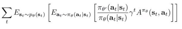
Let this quantity be $\mathcal{L}(\theta’)$. If we can show that $J(\theta’) - J(\theta) \approx \bar{A}(\theta’)$, then we can just set $\theta’ \leftarrow \arg \max_{\theta’}\mathcal{L}(\theta)$ because it maximizes the expression $J(\theta’) - J(\theta)$. But is this quantity close to the real quantity?

Bounding the state marginal differences: deterministic example

We claim that $p_\theta(s_t) \approx p_{\theta’}(s_t)$ when $\pi_\theta \approx \pi_{\theta’}$. Let’s start with the toy case where $\pi_\theta$ is deterministic. We don’t assume that $\pi_{\theta’}$ is deterministic. Rather, we assume that

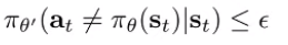
which is a definition of closeness. With this definition, we can write the state marginal of $\theta’$ as a convex combination of $p_\theta(s_t)$ (when the policy makes no mistakes for $t$ steps and $p_{mistake}(s_t)$ (when anything else happens). Naturally, the distribution is

Let’s assume that we don’t know what p_mistake is. This is reminiscent of the imitation learning analysis we did. And as before, we can write a total variation divergence bound.

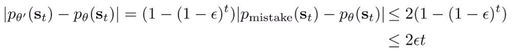
And we use an exponential identity to show that it is finally upper bounded by $2\epsilon t$. This shows that $\epsilon$ decreases, the distributions get closer.

Bounding the state marginal differences: general derivation

We now claim that $p_\theta(s_t) \approx p_{\theta’}(s_t)$ when $\pi_\theta \approx \pi_{\theta’}$ and it is true for any $\pi_\theta$. We revise our definition of “closeness” to use the total variational divergence. We can also use an expectation difference (like KL), but this derivation is simpler

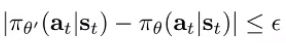
We use one important lemma: if $|p_X(s) - p_Y(x)| = \epsilon$, there exists some joint probability $p(x, y)$ where the marginals match and $p(x = y) = 1-\epsilon$. As such, we claim that $\pi_{\theta’}$ takes a different action than $\pi_\theta$ with probability at most $\epsilon$.

And this brings us back to the deterministic derivation, which means that we get the same bound.

Bounding objective values

Now that we can bound the state marginal differences, can we make any progress on bounding our objective values, which is what we wanted?

To do this, let’s derive a general bound of the expectation of a function under two distributions with bounded differences. We start by making a pretty loose bound.

This bound is true because you’re just saying that $p_{\theta’}, p_\theta$ have a certain point-wise distance, and the total variational divergence is just the sum of the pointwise differences, allowing us to pull it out of the summation.

Now, you can plug in the upper bound we derived previously,

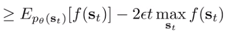
So as long as $f$ is bounded, you can make the expected values arbitrariliy close. Now, let’s plug this back into our original objective:

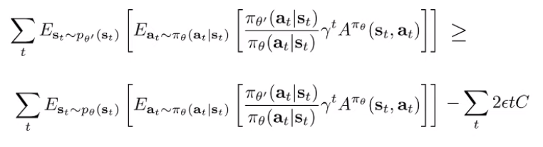
where $C$ is the largest possible value of the inside of the expectation. This $C$ is $O(T r_{max})$, which is derived by noticing that the advantage is bounded by the maximum reward. If we have infinite timesteps with discount, we have $O(r_{max}/(1 - \gamma))$.

Monotonic improvement ⭐

We’ve just created a lower bound to the $J(\theta’) - J(\theta)$ objective using tractable terms. So a good RL algorithm will just try to keep this value non-negative

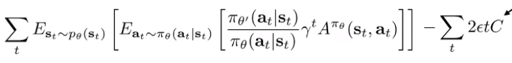
We can define some $\epsilon$ as a function of the maximum reward to keep this statement non-negative. Recall that we want to keep the statement non-negative because it is a lower bound to $J(\theta’) - J(\theta)$. if this is non-negative, then we know that the new $\theta’$ will be at least as good as the current $\theta$.

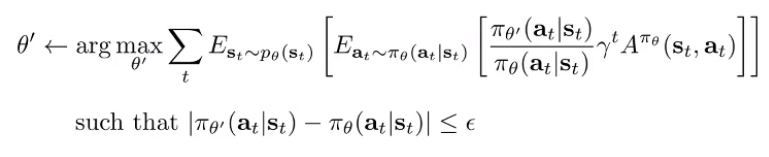
It shows us that as long as we keep $\pi_{\theta’}$ close to $\pi_\theta$ with a well-chosen $\epsilon$, then we have a good shot at optimizing the RL objective.

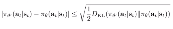
And you can use the fact that total variational divergence is related to KL, so you also get a KL constraint too

Implementing Trust Regions

Concretely, this loss function $\mathcal{L}$ is something you evaluate at your current $\theta$, and then you take a gradient step to make your new $\theta’$. If done correctly, this surrogate objective will be very close to the RL objective and you end up improving the policy.

As a side note: when you start at $\mathcal{L}(\theta)$, the importance weight is not a constant. Namely, the denominator is a constant (what you start with) but the numerator is a variable (what you intend to change). They start out being $1$, but it is not always $1$. This is why the gradient exists.

Trust region as constraint

You can just write out a Lagrangian expression

and then you can use standard dual gradient descent techniques for constrained optimization. This gives rise to Trust Region Policy Optimization (TRPO)

Trust region as regularizer

We can also treat the constraint as a regularizer, which gets you

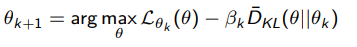
which effectively treats the kl term as a regularizer. We change the $\beta$ to enforce a target KL distance.

• Algorithm (adaptive weighting)

  

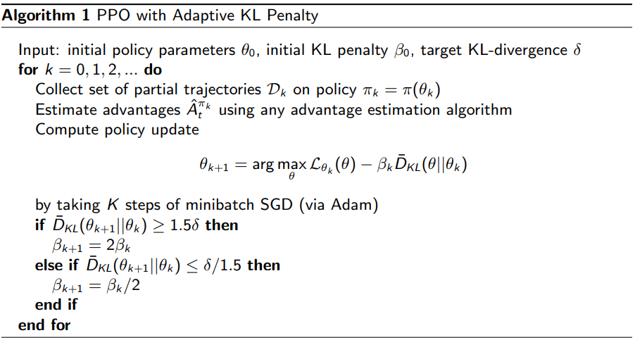
Implicit trust region

We can be even more primitive. Note that the only place where $\pi’$ is involved is the importance weight. So, you can just clip the importance weight. If you clip the importance weight, there is no gradient incentive to change $\pi’$ past a certain point, achiving an implicit trust region. This is the idea of Proximal Policy Optimization (PPO)

• Algorithm (clipped)

  

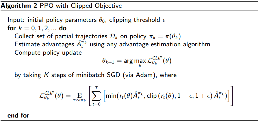
Natural Gradients

You can also use a natural gradient approach to directly influence the gradient descent process to work with the constraint. We start by computing the derivative of the main value

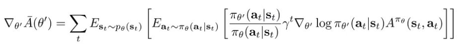
^^look at this carefully; it’s an unconventional formulation, but if you write out the gradient inside, you’ll see why it’s true. The gradient at $\theta’ = \theta$ is just the normal policy gradient.

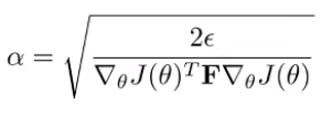
But we can’t just step the gradient directly, because $\theta$-space is not the same as $\pi$-space. You need to use a natural gradient that works in this $\pi$-space. See the conditioned optimization section above for more details. You end up approximating the KL with Fisher Information matrix $F$, and your final update becomes

and you can derive the $\alpha$

The key upshot is that natural gradients + policy gradient is intimately related to trust regions. In fact, the objectives decompose to the same thing.