Actor Critic Algorithms

Tags	CS 285Reviewed 2024

Suggested Readings

Moving toward actor-critic algorithm

In policy gradient, we weighted the likelihoods by the return. As we discussed in the policy gradient notes, we can replace the Monte Carlo return estimate by a critic function that models this return. This is helpful because monte carlo is high variance.

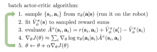
The control variate (baseline) is the average return, which can be interpreted as the value function. So, the optimal estimate is $Q(s, a) - V(s) = A(s, a)$ , known as the advantage function. Putting this all together, we get the generic actor-critic algorithm:

💡

note that actor critic is generally on-policy

Fitting the Models

From classic RL, we know a lot about how we can fit Q and V. We can train Q and V through bellman backups; they are also defined easily in terms of each other. Because we care about advantages, it might be best to fit $V$ , because we can define

A^\pi(s_t, a_t)\approx r(s_t, a_t) + V^\pi(s_{t+1}) - V^\pi(s_t)

V is more convenient to learn too, because it doesn’t depend on actions.

Modifications

We’ve talked about ways of working with bias-variance tradeoff with value functions, like eligibility traces and N-step returns. Look at those notes for such applications.

Practical Choices

Architecture

We can use two neural networks, one for values and one for policy. This is relatively simple and stable to train. However, there are no shared features between the actor and critic, so it’s not as efficient.

You might also use one trunk and two separate heads for the policy and the value. This is harder to train.

Batches

A vanilla online on-policy actor-citric algorithm may not be a good idea. The updates work best if you have a batch. To accomplish this, you can use multiple workers

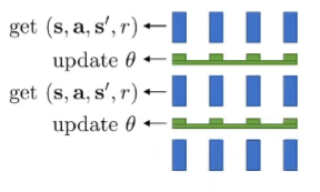
You can also make it asynchronous. This can cause some distribution shift as some transitions are from older policies. In practice, however, this is generally fine.

Removing the on-policy assumption (TO MODIFY)

☝

tl;dr you need to use a Q function

You can just sample from a replay buffer. This removes the on-policy component, but we need to change the algorithm. If you were to just sample from a replay buffer, you wouldn’t have the right target value due to an invalid $a’$ that your policy may not be doing anymore, and the policy gradient isn’t taken under the right expectation.

To get the right target value, you can try using a Q function instead. The main problem is that the sampled $a_t$ may not be what the current actor would do. The Q function explicitly considers $a_t$ , which means that it doesn’t need to be sampled from the current $\pi$ . To compute the value function, just take the expectation over the current policy (or Monte carlo estimation)

To get the right expectation for the policy gradient, we just sample from the current policy $a_i^\pi$ (denoted as $a’$ , instead of using $a_i$ from the buffer)

In practice, we also plug in the Q function directly into the policy gradient. It’s higher variance, but it’s more convenient. And we can sample more actions easily because there’s no simulation need.

So what we have here is an online AC algorithm that can use a replay buffer to continuously improve itself with large batches. This is possible thanks to the Q function.

There is one problem, which is that the state marginal is not from the current policy. However, there’s not much we can do. And ultimately, the distribution is broader than what we want, so the problem is more challenging but we are not missing out on anything.

Critics as Baselines

Previously, we talked about using the critic as an estimation of the returns in the policy gradient. This is one way of using the critic. It lowers the variance drastically, but it is not unbiased.

Alternatively, we could use the original policy gradient formulation but use the critic as a baseline.

State-dependent baselines

The estimator of the PG is unbiased when we subtract any constant or state-dependent baseline. So, why don’t we just subtract the value function?

Action-dependent baselines (control variates)

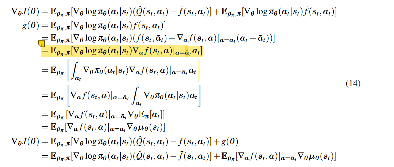
We can reduce the variance further if we use state and action-dependent baselines, known as control variates. A common choice is to subtract the Q function.

Unfortunately, we can no longer use our original proof to assert that such baselines impart no bias. It turns out that you need to account for an error term, and once you do, you get this gradient

The first term is good, but what about the second term? Well, the second term can be evaluated easily, because you don’t need to execute in the environment. So you can actually get closed form or very low variance. This whole method is known as Q-prop.

Derivation of equation (splitting and taylor approximation, taken from Q-prop paper)

Aside: Discount factors

If we have an infinite episode length, we always push up our value function. This can cause value function explosions. To help with this, we use a discount factor. The idea is that it is better to get rewards sooner than later

Theoretically, it just means that the MDP has an additional “death state” that you have a chance of falling into with probability $(1-\gamma)$ that always have reward 0.

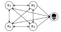
Policy gradients and discount factors

We have two options of using discount factors in policy gradient

Option 1

Option 2

Option 1 is the critic formulation (i.e. you’re using a single-sample estimator of the critic). Option 2 is similar, but note that the exponent on the $\gamma$ doesn’t start at 0; it start at $t - 1$ . So the further along you are, the less the returns matter. tl;dr option 1 downweigh rewards in the future. option 2 downweighs rewards and decisions in the future.

Which version is the right one?

option 2 is consistent with the idea of the death state: your decisions right now are more important than later.

option 1 is more common: want to use the discount to get finite values, but we want solutions that cares about the entire future (so we want something with more foresight)