Unconstrained Minimization

The idea is very simple. Given a convex function, can we minimize it?

So because it is convex, the optimality condition is $\nabla f(x) = 0$. If you have a closed-form expression, minimizing this is the same as solving $n$ equations with $n$ unknowns.

Now, generally this is very hard (because it’s not linear), but if you have a convex quadratic, we can solve the gradient exactly using simple linear algebra.

Strong convexity

A function $f$ is strongly convex on a set $S$ if we have

We can also say that $f(x) - (m/2)||x||_2^2$ is still convex.

Stronger inequality

We know that the taylor expansion is

and when we put the inequality of the hessian inside, we get

for all $x, y \in S$. This gives us a nicer upper bound on a new point $y$ than convexity does alone (when $m = 0$, you’re left with the standard convexity inequality).

Convergence bounding in $f$

You can obtain the bound

This tells us something important: if the gradient is small, we are close to optimality. This feels like a “duh” moment, but it’s important that we see this in a mathematical form. Note that the larger the curvature, the closer we get. It helps because we can stop the optimization when we reach an acceptable error.

• Proof (lower bound)

  We can find the $y$ that minimizes the lower bound, and you’ll get $\tilde{y} = x - (1/m)\nabla f(x)$, which means that if you plug that in, you get the absolute lowest bound:

  

  which tells you that any optimal point $p^*$ must also be greater than that.

  

  and if you rearrange things, you’ll get

  

Convergence bounding in $x$

You can obtain the bound

• Proof (using the lower bound)

  We can apply a similar bounding technique targeting the inputs

  

  where the second inequality is Cauchy-Schwartz. We use the fact that $p^* \leq f(x)$, and plugging that back in, we get

  

  which yields the final inequality

Iterative Methods

For other functions, we use iterative methods, where you make a sequence of points where you hope that

initial point and sublevel set

We do care about the initial point $x^{(0)}$. It must be in the domain of the function (duh), and the sublevel set $\{x | f(x)\leq f(x^{(0)})\}$ must be closed. This is important because if we have a function that decreases asymptotically toward some minimum, our iterative method will never converge.

The second condition is hard to verify, but we can also just prove the general case that all sublevel sets are closed.

• If we know the epigraph is closed

• if we know that the domain of $f$ is all of $R^n$

• If we know that $f(x)→\infty$ as we approach the boundary of the domain (known as a barrier function)

Gradient Descent

The gradient descent method is pretty straightforward:

We can guarentee that $f(x^{k+1})< f(x^k)$, hence the name. By convexity, we know that this inequality implies that $\nabla f(x)^T\Delta x < 0$, i.e. the direction must go against the gradient.

Line searches

The question becomes: what is $t$? It can be just a constant, but can we do better?

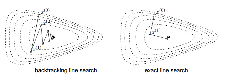
The exact line search option just sets

While this typically yields the best option, it can be slow and maybe even intractable.

The backtracking line search uses parameters $\alpha \in (0, 1/2), \beta \in (0, 1)$. We start with $t = 1$, and then we keep multiplying $t = \beta t$ until

Intuitively, we start by overstepping and then we step back until we fall below a certain estimate.

The diagram above shows the function in the direction of the chosen line, and the two dotted lines show $\alpha t$ (the starting point) and the actual $t$.

The actual algorithm

Convergence analysis

For strongly convex $f$, it is possible to show that

which means that we have exponential convergence. This is a simple algorithm but it can be slow. Let’s investigate this more.

If we have an “ill-conditioned” quadratic shape, then the algorithm will “zig-zag” as it moves to the optimal

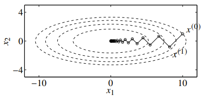
This also depends on what sort of algorithm you pick

Steepest descent method

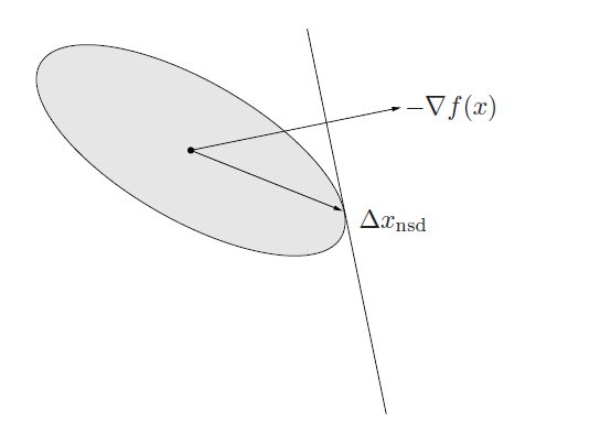
Gradient descent was good, but it operated mostly under a Euclidian norm. Turns out, the zig-zagging problems were caused by improperly assuming that we could use the Euclidian ball. This time, we are defining the normalized steepest descent using some other norm

Depending on the norm, your final $\Delta x$ may not be pointing in the same direction as $\nabla f$. We do know that it is in the halfspace $\nabla f^Tx \leq 0$ because otherwise it would be increasing, but there’s a great deal of jurisdiction. Visually, you can imagine sweeping the plane $\nabla ^Tx$ until it touches the edge of the unit ball.

• L2 norm recovers the gradient descent

• L1 norm recovers coordinate descent

• The quadratic norm ($\Delta x_{sd} = -P^{-1}\nabla f(x)$) recovers a skewed sort of stepping (see visual above)

• you can also choose to use the Hessian (and there are some interesting connections to Newton’s method)

The choice of norms can change the convergence properties quite a lot

Newton’s method

Newton’s method is similar to gradient descent in that it makes an approximation, but this time, it makes a second-order approximation

Visually, it looks like this

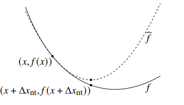
So a newton step is

You can also interpret this as taking a steepest descent direction by using the local Hessian as the norm.

Affine invariance

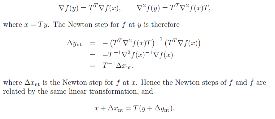
Newton’s step is independent to linear or affine changes of coordinates. This is helpful because then you don’t need to tune any hyperparameters that are specific to one scale

• Proof

  

Newton Decrement

We define the Newton Decrement as

This quantity helps for analytical purposes and it also helps us determine when to stop.

If we define $\hat{f}$ as the quadratic approximation centered at $x$, then we have

by construction (you should show it for yourself). This helps us estimate the proximity of the current $x$ to the optimal point $p^*$. Intuitively, $\lambda(x)$ just tells us how much more do we need to move (and we scale using the inverted hessian because it’s part of Newton’s method).

This is also the norm of the Newton step in the Hessian norm

and it is also the directional derivative in the Newton direction

The actual algorithm

Now, practically speaking, you don’t necessarily want to minimize the quadratic approximation every time. Instead, you treat this $\Delta x_{nt}$ as another step direction, and you still search over the $t$

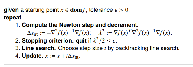
Here’s the really cool part: you actually don’t need to worry about scale; this method is affine-invariant, meaning that if you scaled the variables by some amount, you will converge in the same time, no changes needed.

Convergence analysis

If we have L-lipshitz continuity, then there are two distinctive convergence zones.

This tells us that we get a linear decrement at first, and then we get a quadratic decrement. In general form, we have

Unfortunately, this bound is not affine-invariant (whereas the algorithm itself is)

Self-concordance

Self-concordance is a tangential topic that we touch upon, but it has some cool implications. The previous bounds we proved on Newton’s method wasn’t scale invariant. It turns out that if you can show that

then the function is self-concordant. Some examples include linear and quadratic functions, negative logarithm, and $x\log x - \log x$.

Self-concordant calculus

If a function is self-concordant, it is preserved under positive scaling and composition with affine function. If we have a convex $g$ such that $|g’’’(x)|\leq 3g’’(x)/x$, then the following function is self-concordant:

examples of self-concordant functions from these composition rules include

Convergence analysis

It turns out that you can derive convergence bounds for self-concordant functions of the form

which is affine-invariant. There is a lot more complicated math here, but we’ll leave the result be for now.

Implementation of Newton’s method

In each iteration, we are evaluating derivatives and solving the expression $H\Delta x = -g$, where $g = \nabla f(x), H = \nabla^2 f(x)$.

At first glance, it seems scary that we’re computing the hessian and inverting. For an unstructured system, this is $O(n^3)$ through Cholesky factorization

If there is structure in the hessian, we can reduce the complexity even further.