Maximum Likelihood Estimation

The idea here it to choose from a family of probabilities to maximize the likelihood of seeing some observe data. If $\log p_x(y)$ is convex in $x$ for fixed $y$, then the objective is a convex optimization problem. Note that this is not the same as $p_x(y)$ b eing log-concave in $y$.

Variants

If you have linear measurements with IID noise, i.e.

then your density is

which becomes your objective. Commonly, the noise can be gaussian:

which yields a least-squares solution. If you have Lapalacian noise, you get a L1 norm solution

So this tells us that MLE estimation has some intimate connections to regression and other fitting methods. MLE with gaussian noise is just L2 fitting.

Logistic regression

You can parameterize the distribution as

If you have $y_1, …, y_k = 1, y_{k+1} = …= y_m = 0$, then you get

And this is concave because log-sum-exp is convex.

Gaussian covariance estimation

If you want to fit a covariance matrix to observed data, then the log-likelihood becomes

where

Unfortunately this is not concave as it is, but if you change variables to let $S = \Sigma^{-1}$, then you get

and this is actually concave. Commonly, this $S$ is the natural parameter in an exponential family.

A variant: if you wanted $S$ to be sparse, add a L1 regularizer to each component of $S_{ij}$.

Hypothesis Testing

The idea is this: given an observation of a random variable, you want to decide if the random variable came from distribution $p$ or $q$. You want to construct some matrix $T \in R^{2\times n}$ with each column adding to one. This decision matrix has $T_{1k}$ being the probability that $X = k$ comes from distribution 1. It defines a random variable that determines which distribtion this sample came from, given this observation.

In the special case that all the elements in $T$ are binary, then we have a deterministic detector .

Setting up the problem

So if you compute $Tp$, where $p$ is the distribution (i.e. the literal density), and you also compute $Tq$, you get a confusion matrix.

It essentially tells you how likely you’ll get false positives and false negatives. Now this is nice because we don’t like false positives or false negatives, so this gives us an objective. In fact, this whole thing is a multi-objective problem

We can scalarize it and get

and this is just an LP with a profoundly simple analytical solution:

In other words, you just compare the densities and you threshold them. This $\lambda$ can be interpteted as a hyperparameter. Notice that the solution is a deterministic detector. Not all solutions are deterministic; some Pareto-optimal detectors are non-deterministic.

Minimax detector

You would have a minimax objective with the false positives and negatives

which is still a linear program because the maximum of linear functions is still convex. But the solution is no longer deterministic

Experiment Design

The setup is this: you have $m$ linear measurements of a quantity $x$ with some measurement errors

and the $w_i \sim N(0, 1)$. You want to make a set of measurements such that your error is “small.” Let’s formalize this a bit. If you do the algebra out and treat the $A$ as a matrix, the least squares estimate of $x$ for a choice of $A$ is

And the error has zero mean with covariance (this is just algebra and stuff)

So our objective becomes minimizing the $E$.

Vector optimization formulation

We can formulate this as vector optimization. So first, we restrict $a_i \in \{v_1, …, v_p\}$ to make the problem more feasible. This means that we can define a new $m_k$, which is the number of vectors $a_i$ that was chosen to be $v_k$. This might be more than one, because there is measurement noise.

This is difficult because of the integer constraint

Relaxed experiment design

We can reparameterize the formulation into a distribution $\lambda_k = m_k / m$ and turn it into a continuous random variable. So the objective now becomes

This is convex, and the solution is a lower bound. You can just round $\lambda_k m$ can give you a good starting point for the problem.

Of course, this objective is actually in matrix space, which may or may not be easy to deal with.

D-optimal design

Instead of having the expectation be the objective, you could also have the objective be the confidence ellipsoids. This gives you a scalar formulation of the objective

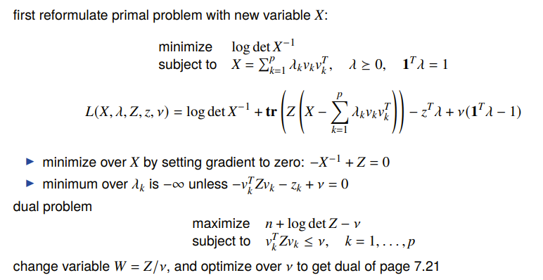
We can find the dual of this problem and it becomes

The intuition is that we make a minimum volume ellipsoid (defined by $W$) that includes all the test vectors.

The notion of complementary slackness states that if we are optimized, then

which tells us that we use vectors $v_k$ on the boundary of ellipsoids defined by $W$.

• Derivation of Dual