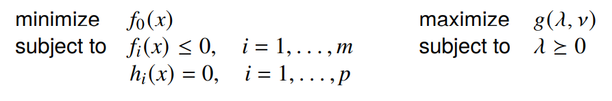
Duality
| Tags | Techniques |
|---|
Lagrangian
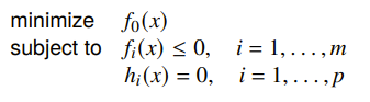
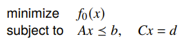
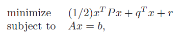
The standard form optimization problem has this format:
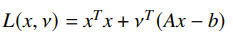
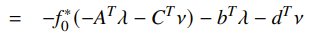
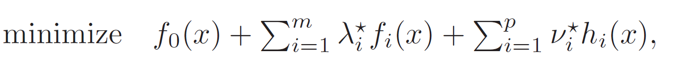
We can construct the Lagrangian as the following equation:
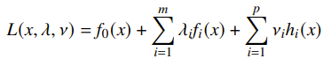
where are lagrange multipliers. Intuitively, you can understand the Lagrangian as treating the constraints as a form of cost and revenue. if you don’t reach the constraint, it can help you reach a lower objective. If you exceed the constraint, you incurr a cost. We’ll talk about how we can extend this to hard constraints later.
Matrix and vectors
If you have a vector inequality, you can usually express this as an inner product with some vector . For example, if you have , then it becomes (think about this for a second).
If you have a matrix inequality, it naturally makes sense that you would compute the matrix inner product, which is just , where is the Lagrange matrix.
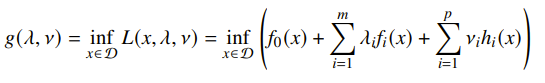
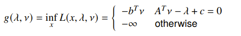
Lagrange dual function
So in the Lagrangian, we introduced the multipliers. This feels weird, and we’re not quite sure about what they do. So we formulate the Lagrange dual function, which looks at how the multipliers behave as the function of the minimization across .
Turns out that this is concave. is an affine function of for each . The infimum of a bunch of affine functions, which is concave. You might find that some values of create unbounded optimziation problems. This has significance that we’ll talk about later.
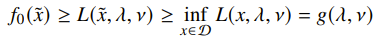
Dual function is a lower bound ⭐
is also a lower-bound on the optimal value of the problem. This is easily proven through the definition. As long as you have a feasible , then the following is true, by properties of and infimums.
If you can find a closed-form expression for this , then you can have a good lower bound on the true constrained optimization.
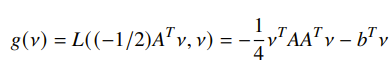
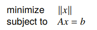
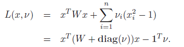
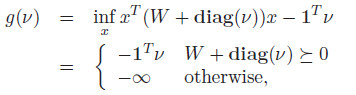
Example: least-norm to linear equations
If we have
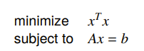
The Lagrangian is
Then you can have a closed form expression for solving the lagrangian

and this gets you a general expression for :
Example: standard LP
If you have
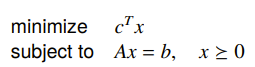
Then the lagrangian is

And because this is affine, we notice that the infimum has a pretty interesting property:
Example: equality constrained norm minimization
If we have
then the dual function also has a special domain
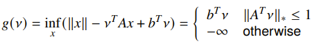
where , otherwise known as the
dual norm.
Example: two-way partitioning problem
If we have
this is equivalent to cutting the vector into 1 and -1, such that some objective is optimized. Turns out, you can have Lagrangian as
And so the dual is
Relationship to Conjugate function
It turns out that there is a pretty neat connection between the Lagrange dual and the conjugate function. Lets say that we had this set of constraints in an optimization problem:
If we write out the dual function, we’ll see
And if we remember the definition of the conjugate function as , you can rewrite the dual as
This is useful because if you know the conjugate of , the dual is trivial to compute.
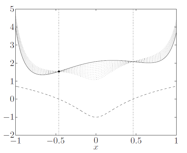
Linear approximation interpretation (the taxation interpretation)
While this has cool mathematical properties, it also has some important intuitive properties. In the hardest case, we have

where the indicator function is when the constraint is violated. This represetns a sort of “infinite displeasure” at violation. The Lagrangian is the same formulation except that the indicator functions are replaced with linear approximators which represent as “soft” displeasure.
So this is a really nice diagram. The solid line is the objective, the dotted line is the constraint. The valid points are between the vertical lines. The “haze” around the solid line is the Lagrangian function with different values of . See how they form a lower bound for everything inside the feasible set?
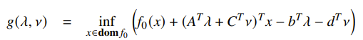
Lagrange Dual Problem
We previously established that the Lagrange Dual provides a lower bound on the optimal value . But what is the best lower bound? In other words, can we get really close to the optimal value? For this, we present the dual problem:
Because is concave, this is a convex optimization problem, even if the original problem (known as the primal problem is not). We denote the dual optimal value as .
We’ll notice an interesting property: there are certain constraints in the primal problem that turn into implicit constraints in the dual problem (i.e. if you don’t follow such constraints, the dual problem will yield negative infinity.
Adding implicit constraints
Make sure to look at the infimum carefully, especially if you’re dealing with an LP. Often, with an LP, you’ll get somethign like . In this case, the infimum goes to negativity infinity unless . Make sure that you add these implicit constraints into your dual function before your blindly take the gradient.
Types of Duality
Weak Duality
The weak duality is just a restatement of our old derivation: . This holds true for any sort of problem (because the dual is a lower bound), and we can use this to find non-trivial lower bounds of potentially difficult problems.
Strong Duality ⭐
The other form, strong duality, is much more interesting. This is when , and it doesn’t hold in general. In general, if you see an LP, you can assume strong duality because of Slater’s constraint. You can also use this as a certificate of optimality. If you have , then both parameters are optimal (because we know that is a lower bound of ).
Slater’s Constraint
If the problem is strictly feasible, i.e. there exists some such that
then strong duality holds. If is affine, we can exclude it from Slater’s constraint. Vacuously, if all is affine, then strong duality automatically holds. IF there are no inequalities, then feasibility is all we need.
Primal and dual relationships
Note that when we started, we had the Lagrangian function
Let’s think about the primal problem. At each feasible , we can say that . This is because if , then the supremum would push everything to infinity. Likewise, if , the supremum could push everything to infinity. As such, the optimal value of the primal problem is
Let’s marinate on this for a second. The primal problem will either be infeasible, or the inner supremum yield ’s that are zero.
Let’s contrast this with the dual problem, which has
Let’s think about this. In some cases, the yields and therefore makes the outer problem infeasible. This is similar to the primal version of the problem.
We know from our previous discussions that is a lower bound for . But what happens with strong duality? Well, we’re essentially saying that
This actually has two very neat interpretations. First, if we think about this setup as a min-max game, this tell us that either player gains an advantage by going first. This is generally not true without strong duality.
Second, this tells us that form a saddle point of the Lagrangian if there is strong duality. In other words,
conversely, if is a saddle point of the Lagrangian, then is primal optimal and is dual optimal.
Geometric Interpretation of Duality
Initial interpretation
Let’s try to understand the meaning of the dual function geometrically. Let’s start with one constraint and an objective function . We can plot the values on the x-y axes with a section for the achievable values of as
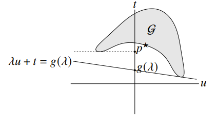
We define the dual function as . Note that we do inf u, t which is implicitly .
Let’s start with the function . This is a set of non-vertical lines of slope . It is minimized when it touches because the level curves are all pointing in one direction (and it’s positive). So the line has value all throughout, so the t-intercept has .
You can start to understand why the lower bound condition is true, and perhaps you can start to visualize which conditions of are required to have strong duality.
Epigraph variation
If we consider the epigraph as part of the valid set (think about this carefully), this gets you a new set . Previously, was a free-floating value that we wanted to minimize. Now, because it’s drawn as the feasible region, we know that the optimal value will occur at the edge of the set , and more specifically, as crosses axis.
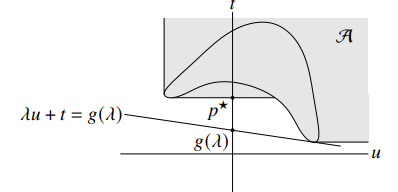
This allows us to formulate the strong duality restriction quite cleanly: if there is a non-vertical supporting hyperplane at , then it is strong duality. This is true for convex problems because is the convex epigraph.
Without getting into too much details, Slater’s condition guarantees that here exists some with , which prevents a vertical supporting hyperplane from forming.
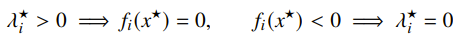
KKT Conditions
The KKT conditions are some properties that tell us neat things about optimality. For convex solutions, satisfying KKT can mean that we satisfy optimality, so it gives us another objective.
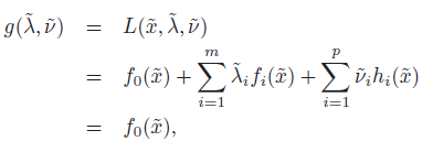
Complementary Slackness
To contextualize the KKT condition, we start with dual optimal definition
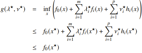
Now, if strong duality is satisfied, then we know that the two inequalities are equalities. There are some interesting upshots we can take from this observation. First, because the second inequality is an equality, we conclude that minimizes (it may not be the only value that minimizes).
We also conclude that
Which brings us to the idea of complementary slackness: at the optimal point, the function is either zero (tight) or we assign no dual weight to it.
Intuitively, this says that if strong duality is upheld, then the optimal value Lagrangian assigns non-zero to constraints that are active.
Mechanics interpretation of complementary slackness
Let’s try to understand complementary slackness. Consider the two cases: if , that means that we are at the constraint and we are held tight by these constraints.
If , it means that we actually don’t really care about this constraint because we haven’t reached it.
If we understand these constraints as different chains that guide an object, the first case is that the chains are taut, and the second case is the chains are loose. Complementary slackness means that the chains are either taut or loose, and that the tension (non-zero ) only happens when the chains are taut.
The KKT Conditions
If we have strong duality, let’s consider the relationship between and . The lack of duality gap states that minimizes over . Therefore, the gradient of at that point must be zero.
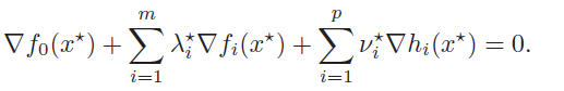
Therefore, we have the following conditions, which are known as the KKT conditions
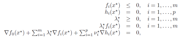
Any must satisfy these conditions for a strong duality setup.
Using KKT Conditions on convex problems
Normally, the KKT conditions are necessary but not sufficient for optimality. But if the primal problem is convex (and strong duality), the KKT conditions are also sufficient.
Proof
The third equality is complementary slackness. The first equality comes from the gradient vanishing and convexity.
Because and ordinarily it’s a lower bound, we know that we’ve reached optimality.
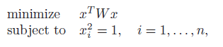
In some cases, it is possible to solve KKT conditions exactly. Many algorithms for solving convex optimization (like constrained Newton’s methods) are just solving KKT.
For example, if you want to minimize a linear-constrained quadratic
The KKT conditions are
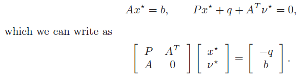
If we solve this linear equation, we get the optimal primal and dual variables.
Solving primal with dual
From above, we know that with strong dual problems, minimizes . So, if you had the optimal , you can solve for the primal by just doing
Note that we are not guarenteeing that is a convex function, so we might have multiple solutions, or no solutions at all. If the solution is not primal feasible, then no primal optimal point can exist.
This structure is helpful if the dual problem is easier to solve than the primal problem.
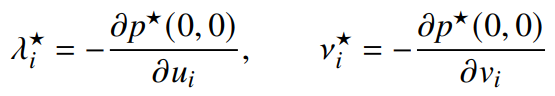
Sensitivity Analysis
In sensitivity analysis, we are interested in how the solution changes as we change some of the boundaries of the constraints. We start with the unperturbed problem
And we can get the perturbed problem and the dual

We can formulate the optimal value as a function of : .
Global sensitivity via duality
If strong duality holds for the unperturbed problem, we can apply weak duality and substitute in the strong duality assumption

So this tell us a lot of interesting things (mostly, we can tell when things get worse becuase it’s a lower bound)
- If we tighten constraint by making , the rate that increases depends on .
- If is positive, then taking will increase
- IF you stare at this for awhile, you’ll see other sensitivities
List
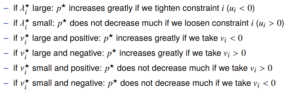
These results remind us about a deeper truth of what the multipliers mean. They are telling us how much we care about a specific constraint, as in, if we made the constraint tighter, how much we would lose.
Local sensitivity via duality
You can take a deeper look at by taking the derivative. We know that
from the global sensitivity result. Unlike the global sensitivity result, local sensitivity is not asymmetric; it tells you exactly what happens to the objective upon perturbation, not a lower bound (because strong duality holds at ).
Proof

Problem Reformulations
A critical important note is that equivalent problem formulations can yield very different duals, which means that reformulations can help if the duals are difficult or too trivial
Common reformulations include
- introduce new variables and equality constraints
- Make explicit constraints implicit, vice versa
- transform objective or constraint functions
Adding new variables and equality constraints
Adding constraints in general can make your dual more interesting. As a very didactic example, if you want to minimize the dual is constant. Therefore, it helps to introduce a new variable and an equaltiy constraint , which gets you a far more intersting dual.
Example: reformulation
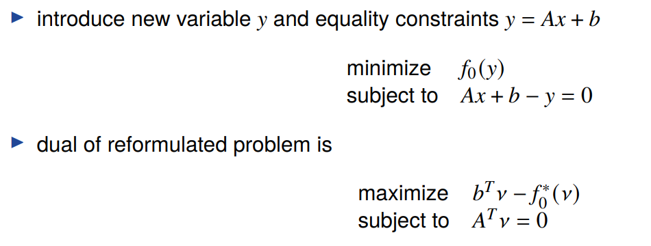
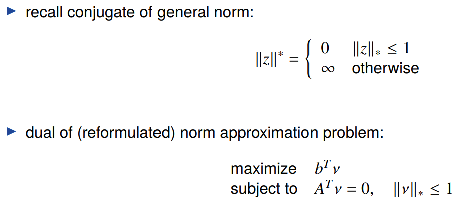
Example: where is a norm
Theorems of Alternatives
The Theorem of Alternatives looks at feasibility problems specifically. We look at two systems of inequality/equality constraints. This can be more than one constraint per system.
- A
weak alternativeis when no more than one system is feasible. This can include the case when neither is feasible.
- A
strong alternativeis when exactly one of them is feasible all the time. Note that Strong alternatives are necessarily weak alternatives too.
These help because we can implicitly prove that something is not true if you can show that the alternative is true. Or, if you have a strong alternative, you can prove that something is true by showing that the alternative is false.
Weak Alternatives for Feasibility Problems
Recall that we setup a feasibility problem as the objective being . The duality therefore becomes
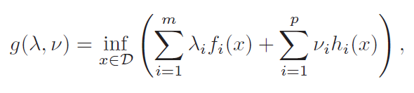
Now this is a really special structure, because is a homogeneus function of . Therefore, this is the solution to the dual problem:
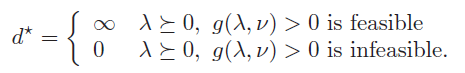
We also know that , which means that if is infinite, then the optimal value of the primal problem must be also infinite, meaning that it’s infeasible. Therefore, these two things are weak alternatives:
- , is feasible
- is feasible
If you have strong duality, then (with certain conditions), strong alternatives holds.
Strong alternatives
When the original inequality system is convex, sometimes weak alternatives become strong alternatives. In general, however, you can’t say too much. Don’t assume strong alternativves
Strong alternative example
The system does actually have a strong alternative
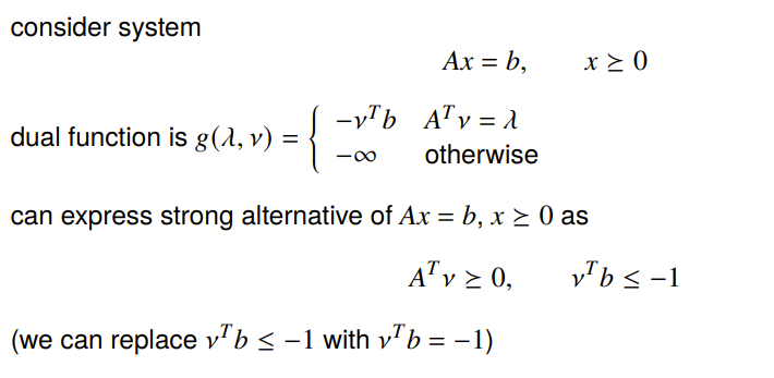
Farka’s Lemma
Farka’s lemma concerns a specific set of nonstrict linear inequalities. The following are strong alternatives:

Proof: LP duality
We have the problem and its dual
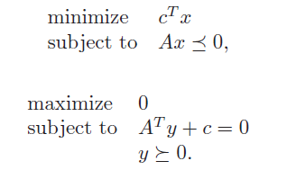
Strong duality holds, so the feasibilities are linked.
Deriving alternatives
You can derive alternatives by doing the following:
- Computing dual
- Find the cases of such that .
- Because is positive homogeneous, we can also write it as .
Because this will tell you that the original problem is not zero, and therefore, it is not feasible
Using alternatives
If you have weak duality and you want to show that something isn’t happening, it is sufficient to show that the alternative is possible (feasible). This can be helpful to plug inti CVXPY.
More specifically: this is an incredibly useful tool! Feasibility problems are “one example” sort of deals. But if you have a set of constraints that you want to be violated (i.e. inverting feasibility), then it is sufficient to find the alternative and show feasibility. Tl;dr it can turn a universal proof into an existence proof.
But importantly, unless you’re given permission to solve a reduced problem, you need strong alternatives to assert that you’re actually solving the same problem
Brief note on dual feasibility
Often when you work on these problems, you take a primal problem → dual problem → feasibility problem. If you take the dual of this again (perhaps to find a strong alternative), you may not get back the primal problem. The dual operation is not subject to the transitive property