Proof Tips

Showing convexity

A set is convex if and only if for every $\theta \in [0, 1]$ and $x_1, x_2 \in S$, we have $\theta x_1 + (1-\theta)x_2 \in S$. To show convexity, you can

• apply definitions (hardest)

• use convex functions (epigraph, sublevel set)

• show that the set is obtained through convex-preserving mappings

• show that it is a subspace (a stronger condition)

Showing something is not convex

• find counterexample (simplest)

Avoid applying definitions as they are often messy

General patterns

• for convex functions, the epigraph is convex and the inverse (outside epigraph) is not convex.

• If $f(x) \leq \alpha$ is convex and $f(x)$ is affine, both inequlaities are convex. If $f$ is concave / convex, it’s not possible to have convex sets with both inequalities

Showing something in a set

A set typically has certain rules. You want to show that something (like a convex combination) can be written in a similar format and satisfies these rules. This is sufficient to showing that something belongs in some set.

Affine and Convex Sets

Lines and line segments 🐧

If you have any points $x_1, x_2$, then you can define a line as

If $\theta \in [0, 1]$,l then this is a line segment. If you don’t constrain it, then you get a line.

Affine Sets 🐧

A set $C$ is affine if for all $x_1, x_2 \in C$, then $\theta x_1 + (1-\theta)x_2 \in C$. Visually, these are typically lines or planes or larger subspaces. We can extend this to any arbitrary number of coeficients, as long as the coeficients add to 1 (no constraints about the negativity of the coeficients, so the coeficients are not bounded).

If we have a set of points, the affine hull is the set of possible affine combinations of these points. Often, they look like a hyperplane or a subspace containing the points, shifted away from the origin by some amount. We denote this as $aff(C)$.

Affine sets and subspaces 🚀

By definition, subspaces are affine sets. But are all subspaces vector spaces? Well, not really. So vector spaces needs to contain zero, and we don’t guarantee this in $C$. But what if you had some $x_0 \in C$? Can we say something about the space $C - x_0$? Actually, you can! In fact, we claim that $V = C - x_0$ is a subspace.

• Proof

  We just need to show that it is closed under addition and scalar multiplication. We use the fact that $v_1, v_2 \in V$ means that $v_1 + x_0, v_2 + x_0 \in C$. Therefore,

  

  because each of the components $v_1 + x_0, v_2 + x_0, x_0 \in C$ and the coefficients add to 1. And because $\alpha v_1 + \beta v_2 + x_0 \in C$, we conclude that $\alpha v_1 + \beta v_2 \in V$.

  We can make a similar proof for scalar multplication.

The critical upshot is that $C = V + x_0$, which means that any affine set is just a shifted version of a subspace!

The solution set to $Ax =b$ is an affine set and conversely, every affine set can be expressed as the solution set to linear equations.

• Proof (just algebra)

  

Affine dimension, relative interior (extra)

The affine dimension of a set is the dimension of the affine hull.

We define the relative interior of an affine hull intuitively as the space enclosed by the points. Don’t worry too much about this rigorous definition for now.

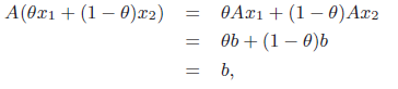
Convex Sets & Convex Combinations 🐧

A convex set is basically an affine set, except that $\theta \in [0, 1]$,and for the multi-coefficient condition, we have $\sum_i \theta_i = 1$. The point $\sum_i\theta_i x_i$ is the convex combination of $x_1, …, x_k$. Like with affine, a set is convex if and only if it contains every convex combination of points.

Convex combinations are generalizable to infinite sums, integrals, and probability distributions. This is helpful for many cases, like generalizing properties to expectations.

The convex hull is the set formed by all possible convex combinations of the points in a set. These convex combinations may not be unique. It is denoted by $conv(C)$.

Intuitively, convex hulls look like you put cling wrap around the shape or set of points.

When you are showing if a set is convex but not affine, you might arrive at some non-negativity property of $(1-\theta)$ or $\theta$.

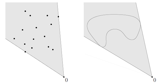
Cones 🐧

A set $C$ is a cone if for every $x\in C$ and $\theta \geq 0$, we have $\theta x \in C$. Note that this could just be a bunch of lines spreading out from the origin. If you wanted an actual “cone” shaped space, you need the additional condition of convexity. If we have convexity, we have a convex cone, meaning that $\theta_1 x_1 + \theta_2 x_2 \in C$.

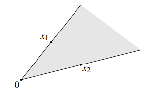
A conic hull is just all $\sum_i \theta_i x_i$ where $\theta_i\geq 0$. This is also the smallest convex cone that contains $C$.

A cone is just a restricted subspace where the coefficients must be positive. Any subspace can be a cone; just put two copies of the vectors facing in opposite directions.

Examples of Convex Sets

Some degenerate examples

• empty set must be affine and convex by vacuous t ruth

• Lines are affine, and if they pass through zero, it is also a cone (if you have a degenerate cone with $x_1, x_2$ pointing in parallel but opposite directions.

• Line segments are convex but not affine unless it’s a point

• A ray is convex, not affine. If the base is $0$, then it is a cone

• Any subspace is affine (and therefore convex) as well as a convex cone.

Convex hull

This just creates a convex hull that surrounds a set of points

Hyperplanes, Halfspaces

A hyperplane is the solution to

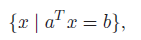
This is the set of points with a constant inner product to $a$. But what does this mean? Well, it’s much easier to see it as

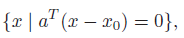
where $a^Tx_0 = b$. In this case, it’s clear that we want the set of points $x$ such that $x - x_0$ is perpendicular to $a$. You can also write this as $x_0 + a^\perp$. Note how this $x_0$ can be multiple things but the easiest is the point colinear to $a$

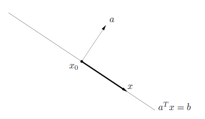
A hyperplane divides $R^n$ into halfspaces, which is the solution to

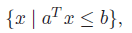
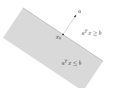
Halfspaces are convex but definitely not affine.

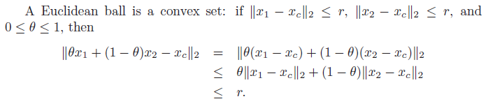
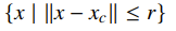
Euclidean balls and ellipsoids

We define a euclidian ball as literally a sphere in R2.

And the generalization is the ellipsoid

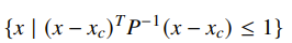
Note that $P \in S_{++}^n$, i.e. symmetric positive definite. The lengths of the semi-axes are $\sqrt{\lambda_i}$

• Proof of convexity (triangle inequality)

  

If $P$ is semidefinite, there may be degenerate axes, but it is still convex.

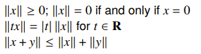
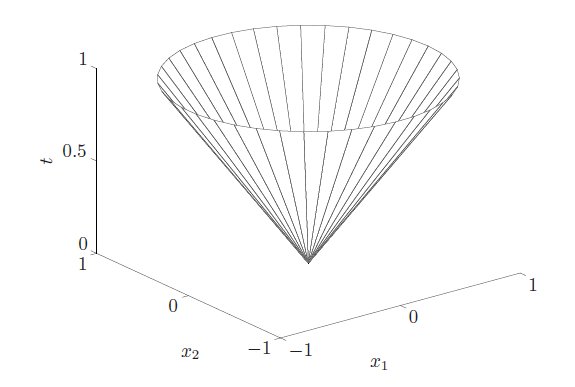
Norm Balls, Norm Cones

Norms are anything that satisfies non-negativity, scaling, and triangle inequality

You can define a norm ball as just the ball using this norm

And the norm cone as basically a norm ball that varies with one extra axis, the radius. If the norm is euclidian, it’s called the second order cone or the Lorentz cone.

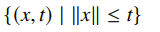
It’s called a cone because it can look like a cone. Think of sweeping a circle upwards and larger.

Polyhedra / Polytope

A polyhedron is just a solution set to a finite number of linear equalities and inequalities. Polyhedra include affine sets and other infinite sizes, although if we get examples that are bounded on all sides, then we have a polytope.

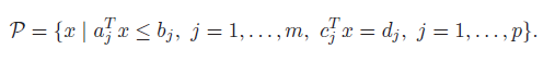
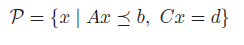
A convex hull of a finite set is a polyhedron, but it’s not easy to express it in the inequality form. You may need more points to describe a polyhedron as a convex hull, as compared to using inequalities.

Positive Semidefinite Cone

Now we’re getting into some weird places. If $S^n$ is the set of symmetric $n\times n$ matrices, then the set $S_+^n$ is a convex cone. Meaning, that if $A, B \in S_{+}^n$, then $\theta_1 A + \theta_2 B \in S_+^n$.

• Proof (definition)

  

Operations that Preserve Convexity

Forward and inverse images

Let’s clear up image and reverse image a bit more.

• If you’re interested in image: you have some original set $S$ and you’re applying $f$ to it, and after applying, something clean happens
  • alternative interpretation: if $S$ is the original set, then $f(S)$ has nice properties
  • We say that this $f(S)$ is the image of $S$.

• If you’re interested in reverse image: you have some original set $S$ that you can apply $f^{-1}$ to and after applying, something clean
  • Alternative interpretation: you have a set with nice properties $S’$, and applying $f(S’)$ gets you $S$
  • You say that this $S'$ is the inverse image of the $S$.

• Commonly, if you have some $h(y)$ constraint that is simple, and you have some $g(x)$ that is less simple, and you can say that $f(y) = x$, then this is an inverse image situation. You have the set $y \in S'$, and applying $f$ gets you the variable $x$ nad the set $x \in S$. Note that you are not changing the criteria; you’re just changing the mapping.

• If you have some $h(y)$ constraint that is simple and you have $g(x)$ that is less simple and you can say that $f(x) = y$, then this is the forward image situation. This is more rare.

Proof tips

You always want to map something back to simple land

• forward images: show that $f(x) = y$, and $h(y)$ is convex

• inverse images: show that $f(y) = x$ and $h(y)$ is convex.

Intersection

Convexity is preserved under intersection, and the proof is really simple. Just use the convex definition and the intersection definition.

This is true for any intersections, including infinite ones. The converse is also true: every closed convex set is an intersection of halfspaces. It is also the intersection of all the halfspaces that contain it.

A common use of intersection: you have some $a = f(t)$, where $t$ is some variable and $a$ is a vector, and your constraint is $a^Tx\leq \beta$. In this case, you take the intersection across all values of $t$ to get you the final convex set.

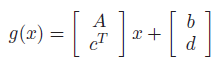
Affine functions

If we transform a space by an affine function $f(x) = Ax + b$, then it is still convex. This is also true for the inverse image of a convex set under $f$, i.e. some $x$ such that $f(x) \in S$.

Examples

• scaling, transformation

• sum of sets, partial sum of sets

• projection

• linear matrix inequality

• hyperbolic cone

Perspective Function

The perspective function $P: R^{n+1} → R^n$ is something that mimics the pinhole perception of an object. A good example is a pinhole camera that projects onto the plane $x_3$.

The perspective function is explicitly defined as $P(x, t) = x/t, t\geq 0$, where $t$ is the dimension that you’re projecting on. Therefore, in R3, we have the projection operator $P([x_1, x_2], x_3) = (x_1/x_3, x_2/x_3, 1)$. We drop this last component because it is always 1.

To use this function, try to look for opportunities to arrange a set in the format $x / t$, and show that this $x$ is convex. Or, you can try having a set $x$ and compute $x/t$ and showing that this $x/t$ is convex. It depends on which direction is simpler.

Linear fractional functions

This is the composition of a perspective function with an affine function. You can write the affine function as a block matrix

and we do this because the last component is special. When we compose $g(x)$ with $P$, we get

and this is the linear-fractional or projective function. You can also interpret linear-fractional function in the form of a matrix $Q$

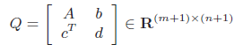
that you apply to vectors $(x, 1)$ and normalize the last component before dropping it. Geometrically, it looks like you’re viewing something at an angle. But more importantly, a lot of different expressions are linear-fractional. They can be helpful for later!

Images and inverse images under linear fractional functions are also convex.

Generalized Inequalities

Proof tips

TODO

Proper Cones

We define a cone to be proper if it is

• convex

• closed (includes endpoints)

• solid (nonempty interior)

• pointed (contains no line, which can happen with a regular cone)

Proper cones and generalized inequalities

You can define an inequality with respect to a proper cone, such that

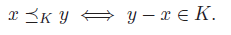
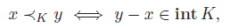
This just means that the partial ordering has a difference that is in a cone.

Note that this is nuanced; it is only a partial ordering. It may be possible to have something such that $x \npreceq y$ and $y \npreceq x$, because if $y - x \notin K$, it doesn’t imply that $x - y \in K$.

Many properties are consistent with normal inequalities

• preserved under addition

• transitive

• preserved under non-negative scaling

• reflexive

• antisymmetric (if $x \preceq y, y\preceq x$, then $x = y$)

• Preserved under limits

Special cases of generalized inequalities

• Positive Orthant: $R_+^n$ forms a cone, and $x \preceq_{R_+^n} y$ corresponds to a component-wise inequality $x_i \leq y_i$. If $n = 1$, we derive the scalar inequality
  • for vectors, there’s a clear example of partial ordering not implying full ordering

• Positive semidefinite cone allows a partial ordering of PSD matrices.

• Non-negative polynomials on $[0, 1]$ allow a partial ordering of polynomials

Maximum and Minimum elements

As mentioned above, generalized inequalities do not impose a linear ordering, which would mean that any two points are comparable. But there is the concept of maximum and minimums, but it gets weird.

$x \in S$ is the minimum element of $S$ with respect to some $\preceq_K$ if for every $y \in S$, we have $x \preceq_K y$. Vice versa for the maximum element. These points are unique, and it means that $S \subseteq x + K$.

$x \in S$ is the minimal element of $S$ with respect to some $\preceq_K$ if for every $y \in S$, we have $y \preceq_K x$ if and only if $y = x$. Vice versa for the maximum element. This is a slightly different definition, and in certain cases it is equivalent to the first definition. However, a key technicality emerges when we realize that certain $y$ is not comparable to $x$ and therefore doesn’t matter. In contrast, minimum elements are comparable to all $y \in S$.

Under this insight, we realize that minimal elements are not unique. A point $X \in S$ is minimal if and only if $(x - K)\cap S = \{x\}$.

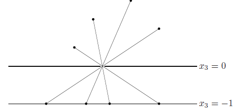
The easiest way of understanding this nuanced difference is through an example of the $R_+^2$ cone.

$x_1$ is the minimum element (the lighter shade i the cone), and $x_2$ is one of many minimal elements.

Separating and Supporting hyperplanes

Separating Hyperplane Theorem

If $C, D$ are non-empty and disjoint convex sets, there exists some $a \neq 0, b$ such that

• $a^Tx \leq b$ if $x \in C$

• $a^Tx \geq b$ if $x \in D$

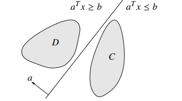
This is not true for non-convex sets. Can you think of an easy example?

Supporting Hyperplane Theorem

Given some $x_0$ as a boundary point of set $C$, a supporting hyperplane is defined as $\{x | a^Tx = a^Tx_0\}$ such that $a^Tx \leq a^Tx_0$ for all $x \in C$. Or, another way to put it: $a^T(x - x_0) \leq 0$, which means that the hyperplane inequality contains the whole set. The equation is satisfied by all points in the hyperplane.

The supporting hyperplane theorem states that if a set is convex, there exists a supporting hyperplane at every boundary point.

Dual Cones

This section is more developed in the textbook but for now, we’ll just use a sneak peek

Dual cone definition

If $K$ is a cone, then

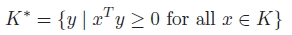
is the dual cone of $K$. Interstingly, $K^*$ is a cone and convex, even if the original cone is not. Geometrically, we can understand $x^Ty$ as a halfspace. If the halfspace contains the cone, then $y$ is allowed. In the picture below, the left is valid and the right is not

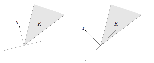
Here are some properties

• $K^*$ is closed and convex

• If $K_1 \subseteq K_2$, $K_2^* \subseteq K_1^*$.

• $K^{**}$ is the closure of the convex hull of $K$, so if $K$ is convex and closed, $K^{**} = K$

There’s some deeper truth, and when we reach function space we’ll see a nice analogy in function land.