Problem formulation tips

Start by finding out what you want to optimize, and then finding out what’s preventing you from taking that to infinity or negative infinity.

A common trick is to take an objective and adding a constraint to make the problem easier. More specifically, it can be helpful to turn a potentially out-of-scope objective and turn it into an in-scope objective with an additional constraint. Or, use an auxiliary variable. See below for two examples

Quasiconvex functions

You can’t optimize quasiconvex functions directly, but you do know the sublevel sets are convex, so you can just find the smallest sublevel set that is feasible.

Indicator functions

If you want to change a restriction into a value, use an infinite-indicator function. If the set is convex, then the indicator function is convex.

Common reformulations for LP

• Infinity norm: $||x||_\infty$ optimization can be formulated as optimizing $t$ such that $-t1 \leq x \leq t1$.

• L1 norm $||x||$ optimization can be formulated as optimizing $1^Ty$ such that $-y \preceq x \preceq y$. This is because absolute value is not in LP form

• Add slack variables if you want to violate the bounds but want to avoid doing so excessively

What doesn’t work

• minimizing a concave function with convex constraints is not convex! This is contrast to maximizing a concave function, which is just the negative of the convex problem.

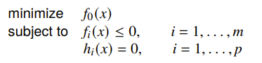
Optimization Basics

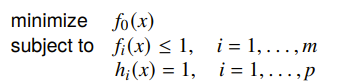
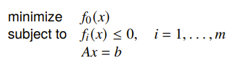
We try to solve this objective:

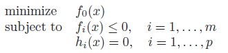
$x$ is the optimization variable and $f_0$ is the objective function.

And obviously, the domain is the intersection of all of the function’s domains. We call a point feasible if it satisfies all constraints. We call a problem feasible if it has at least one such point. The set of feasible points is called the feasible / constraint set. If the constraint functions are convex, then the feasible set is convex (intersection of cvx spaces are cvx)

Formally, we may express our objective as

If the problem is infeasible, the best solution is $\infty$ because the infimum of the empty set is typically denoted as $\infty$.

We call the problem convex if constraints are affine and the objective functions are convex. We call the problem quasiconvex if the objective is quasiconvex and the inequality constraints are convex and the equality constraints are affine.

The variables that make up the constraint variables are part of the optimization problem as well.

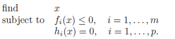
Feasibility problem

Sometimes, we just want to see if a problem is feasible. If this is the case, just define $f_0(x) = 0$. If the constraints have a non-empty feasible set, then the solution is 0. If not, the solution is infinity.

Optimal and locally optimal points

A point is optimal if it is feasible and satisfies $f_0(x^*) = p^*$. We call this set of points the optimal set. If we hit the limit of some inequality, like $f_i(x) = 0$, we say that $f_i$ is active. Otherwise, it is inactive.

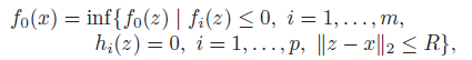
A point is locally optimal if there exists some radius $R$ such that this point is optimal in this radius.

Convex optimization

Remember that convex optimization is only referring to the standard form. There are “abstract” convex optimization problems that have a convex feasible set, but they must be formulated into the standard form to be considered a convex optimization objective.

Optimality properties of convex functions 🚀

Claim: any locally optimal point is globally optimal in a convex function

• Proof (using definitions, contradiction)

  

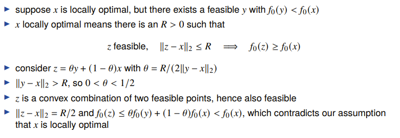
  Visually, it means that if a point if higher than another point, it is impossible to draw a convex function that connects the points without violating the principle of local optimality

This is not true for quasiconvex functions.

Supporting Hyperplane Theorem

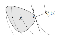
If $x$ is optimal for a convex problem if and only if it’s feasible and

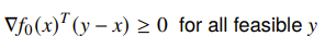
What does does this mean? Well, it’s either zero (at the global maximum) or a supporting hyperplane for the convex set of feasible inputs. This is actually a critical result. It means that we either are globally optimized, or we’re at the boundary.

Therefore, if there is no constraint, this is only satisfied if $\nabla f(x) = 0$.

Relation between convex constraints and convex sets

If you have a convex constraint $f(x) \leq 0$, then the set is convex. Why? Well, you can prove by first principles. If you satisfy the constraint, then

And you have because of convexity and the original constraint

which proves convexity of the set.

Standard Convex Problems

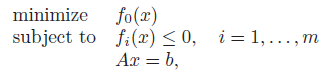
Linear Program (LP)

A linear program is the simplest convex problem, and it means that everything is linear

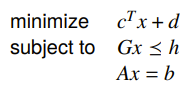
The feasible set is a polyhedron, which means that the optimum point will generlaly be on a point of the polyhedron.

You can cast a piecewise-linear minimization problem as a linear program by using the epigraph problem form (see later section). The key upshot is that if you can make a piecewise linear function that fits even a complicated function, you will be able to maximize it quickly.

Linear programs don’t have closed-form solutions, but they are pretty easy to solve using established methods that we’ll describe later.

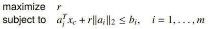
• Example: Chebyshev center of polyhedron

  Given a sequence of linear constraints, can we find the largest inscribed ball? Turns out, we can formulate this as an optimization problem. We notice that the constraints are satisfied at radius $r$ if and only if

  

  which means that we can just formulate this problem

  

If LPs are homogeneous, then the solution is either 0 or $-\infty$.

Quadratic problem (QP)

This one is a step up from linear programs. Instead of minimizing a linear program, we minimize a quadratic program over a polyhedron.

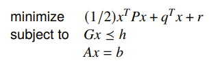
The most common form of quadratic problems are least squares.

• Example: linear program with random cost

  If you have a random cost with mean $c$ and cov $\Sigma$, you formulate it as

  

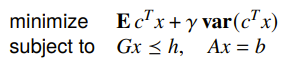
  And it turns out that you can express the variance part as a quadratic

  

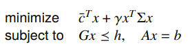
You may also have a Quadratically Constrained Quadratic Program (QCQP), which uses a quadratic constraint. Quadratic constraints are ellipsoids

Second-order cone programming (SOCP)

We can have a constraint that is a cone

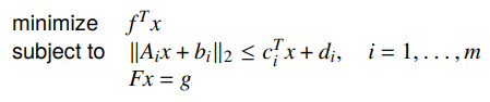
Note that this is not the squared norm, so it can’t be reduced in to a QCQP unless $c_i = 0$. This is a more general form, and it is still convex.

Generally, the constraint $||Ax + b||_2 \leq c^Tx + d$ is a second-order cone constraint.

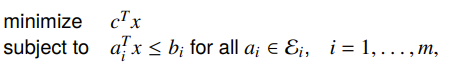
• Example: Robust linear programming

  Here’s an interesting example: what if we wanted an infinite number of constraints within some ellipsoid? In other words: what if we didn’t know what we wanted? Well, we can still write it as a constraint. There are two ways of doing this, both with exactly the same setup.

  The deterministic worst-case tells us that the constraint must hold for all $a_i$ in an uncertainty ellipsoid

  

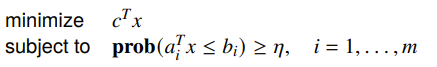
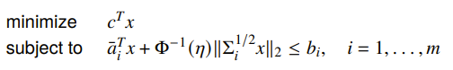
  And the stochastic setup assumes that the constraints $a_i$ is a random varaible and that the constraints must hold with probabiltiy $\eta$.

  

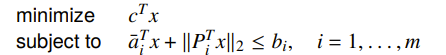
  Turns out, both of these cases reduce down to cone programming.

  For worst-case, the key insight is that the uncertainty ellipsoids are defined as

  

  which means that we just need to have

  

  For the stochastic approach, it turns out that for a gaussian, we can write a closed form expression

  

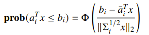
  And we invert this to solve for the constraint:

  

Conic Form Problem

This is when we have our standard affine constraint but the inequality is in conic form.

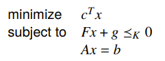
Linear programming is just a special case of a conic form problem.

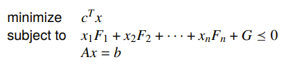
Semidefinite program (SDP)

We can define this cone in matrix space, which allows us to minimize with constraints over matrices

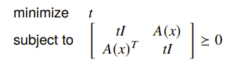
• Example: matrix norm minimization

  If we want to minimize a matrix norm where where $A$ is a combination of different matrices

  

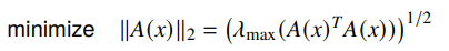
  The equivalent SDP (we’ll just leave this on faith) is

  

Because you are working on matrices, beware of things like PSD (a matrix $X \succeq 0$ means that it is PSD, not that all elements are greater than zero).

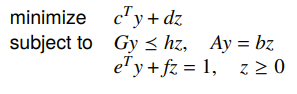
Linear-fractional program

This is when you try to solve

This is a quasiconvex optimization problem because the linear-fractional is quasiconvex. However, you can make it into a linear program by introducing a separate variable $x = y/z$, and this gets you

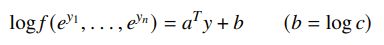
Geometric programming (GP) ⭐

Unlike the examples above, geometric programming is not innately convex. A geometric program is when you have

General tips

If you see a posynomial or a monomial, try letting $y_i = \log x_i$. You might be pleasantly surprised at how far that gets you.

Posynomials

This looks like a convex problem, but $f$ is a posynomial defined as follows:

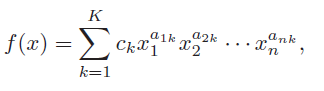
and $h$ are monomials (which are just a single term of a posynomial).The exponents can be anything, but the leading coefficient must be non-negative.

Log-log convexity

Normally, this is not convex, but we can change it into convex form if we apply a change of variables $y_i = \log x_i$. It turns a monomial into an affine function

And the posynomial constraints become a log-sum-exp

Which turns the geometric program into a convex problem. We call this process “log-log convexity” because you replace the variables with the log version, and then you log the outside.

Examples / things that work

Products, ratios, and powers are log-log affine, which is very good when we’re concerned about things with such structure.

DGP

You can build up expressions that are log-log convex incrementally. Just replace the DCP’s “convex” with log-log convex. Here are some good facts to know

• adding is log-log convex because of the log-sum-exp property

• pointwise maximum is log-log convex

Transforming Problems

We saw the standard form in the above section. This means that we are always minimizing, with all constraints using $0$ as the constant. We always have $f \leq 0$, so you may have to negate.

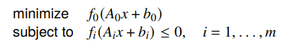
Change of variables

If $\phi$ is one-to-one with a domain larger than the feasible set, then if $x = \phi(z)$, then

is equivalent to

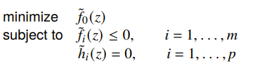
The logic being you can solve in $z$ space and easily teleport back into $x$ space. This is especially helpful because $z$ is simpler (as $x = \phi(z)$), and perhaps it is more likely to be convex.

To do this transformation, you typically start with the $\bar{f}(z)$ and then you build this $f(x)$.

Natural corollaries

• scalar multiplication of constraints

Transforming objective and constraint problems

We have seen how to transform the variables. But what about the functions? Well, if these conditions are satisfied

• $\phi_0$ monotone increasing

• $\psi_i(u) \leq 0$ if and only if $u < 0$ (basically, we capture the crossing point)

• $\psi(u) = 0$ if and only if $u = 0$.

Then, the standard form is equivalent to

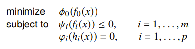
If $\phi_0$ is monotone decreasing, composing $\phi_0(f_0(x))$ can turn a maximization problem into a minimization problem. Commonly, we negate or reciprocal. .

Removing equality constraints

You can implicitly parameterize away equality constraints. If you start with

Then you can get

This is because if you have $Ax = b$, then you can solve for some $F$ and $x_0$ such that $x = Fz + x_0$.

Introducing equality constraints

You can introduce inequality constraints if you have an implicit constraint to start, like this:

because it is the same as

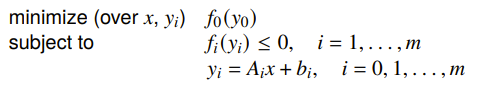
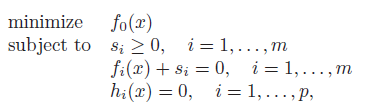
Introducing slack variables

You can also remove equality constraints by introducing slack variables. This allows you to turn inequalities into equality constraints.

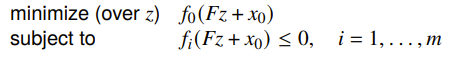
Optimizing some variables

You can always partially optimize the problem; that is legal, and you can complete the other part later.

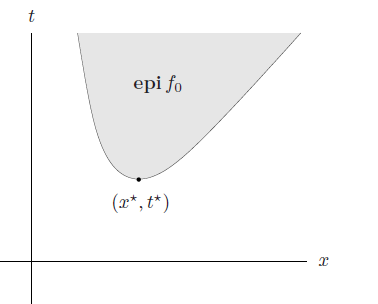
Epigraph problem form

We can rewrite the standard objective as finding the smallest $t$ for an epigraph

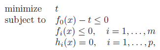
Which has a nice geometric interpretation too. It just means that you’re trying to find the smallest point on the epigraph. The constraints make sure that you stay on the epigraph and within the feasibility bounds.

Implicit constraints

We can also just encode the constraints into the domain of the function

conversely, we can take these implicit constraints of some problems and turn them into explicit constraints.

Convex relaxation

This is when you start with a non-convex problem and find a convex function that is a pointwise lower bound. You also find the convex hull of the constraint set, if it’s not convex to begin with. Then, you optimize this new problem. We call this problem the convex relaxation of the original problem.

• Example: Boolean LP

  The mixed integer linear program takes in two variables, $x, z$. We require $z$ to be binary $0, 1$, but this becomes an NP hard problem. We relax the problem by allowing $z$ to be continuous.

Quasiconvex optimization

Quasiconvex optimization has the form above, where $f_i$ is convex and $f_0$ is quasiconvex. It turns out that solving quasiconvex optimization is just solving a series of convex optimization problems.

Convex representation of sublevel sets

Recall that a t-sublevel set of $f$ is the $x$ such that $f(x)\leq t$. A quasiconvex function has all convex sublevel sets, which means that for every $t$, it’s possible to find some $\phi_t(x)$ whose 0-sublevel set is the same as the t-sublevel set of $f$. More precisely

And this $\phi$ is convex, meaning that at every $t$, we can see if it is feasible easily.

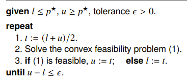
Bisection method

Using this convex representation, we can create a convex feasibility problem

If $\phi_i(x)\leq 0$ is non-empty, then it means that the $f$ is minimized at some point below $i$. This allows us to continue searching only one one half of the divide. This is the bisection method

• Algorithm

  

Multicriterion optimization

What happens if you have multiple objectives?

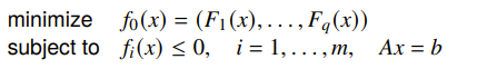
You could have some $x^*$ that simultaneously minimizes each $F$. If this happens, we call the point $x^*$ as optimal. But what if this doesn’t happen?

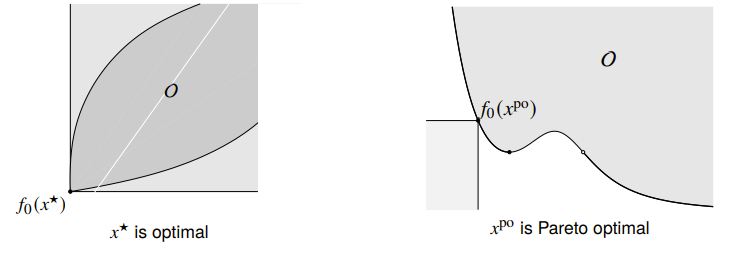
Pareto optimality

We say that a solution $x$ dominates another $\tilde{x}$ if $f_0(x)\preceq f_0(\tilde{x})$ and for at least one $i$, we have $F_i(x)< F_i(\tilde{x})$. So basically it should meet $\tilde{x}$ on all objectives and beat it on at least one.

A feasible $x^{po}$ is Pareto optimal if there isn’t another feasible point that dominates it. You can also say that if $f_0(y)\preceq f_0(x^{po})$, then $f_0(y)= f_0(x^{po})$. Note that $y$ is not necessarily equal to $x^{po}$. There are typically many such points. This idea of Pareto optimality doesn’t exist on single objectives because there’s a notion of strict ordering. Also, as you might see, not all boundary points are optimal, even if the boundary curve is convex.

Relating to our discussion on minimum vs minimal, the Pareto Optimal value is a minimal value of the multi-objective; it may not be the optimal.

Scalarization

You can also just turn the multi-objective into a single objective by summing them togethe

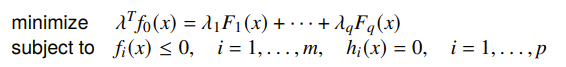
Turns out, if $x$ is optimal for this problem, it is Pareto optimal for the multi-objective problem. We can find different Pareto optimal points by changing $\lambda$. You can understand this $\lambda$ as a hyperplane that sweeps across the output space of $f_0(x)$, and the minimum is the first time the $O$ touches this plane. This also explains why we can get all Pareto optimal points as long as the space is convex.

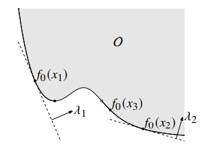
In the graph above, however, $f_0(x_3)$ is not reachable through scalarization, precisely because something is in the way if we try to have a plane tangent to $f_0(x_3)$. (can you visualize why this is the case?)

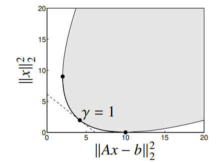
• Example: regularized least-squares

  If you’re tying to regularize a least-squares objective, you’re actually minimizing two things:

  

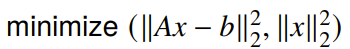
  You can scalarize this objective, and this gives you a convex space. The regularization $||Ax - b||_2^2 + \gamma ||x||_2^2$ is just a choice of $\lambda = (1, \gamma)$.

  

Bonus topics

• Convex-concave optimization: if you have $f(x) + g(x)$ where $f$ is convex and $g$ is concave, you can create an iterative algorithm by linearizing $g$ at $x^k$ and solving $x^{k+1}$, then linearizing $g$ at $x^{k+1}$ and so on.