Proof techniques

Convexity

For convexity, try DCP first, because it’s the easiest. Recall that the composition tricks are sufficient but not necessary, so if they fail, you need another trick that invokes a necessary definition of convexity.

• See if epigraph is convex (may be harder unless there’s a neat trick)

• See if sublevel set is convex (necessary but not sufficient)

• Jensen’s inequality (good for counterexample)

• Second derivative (nasty if multiple variables because it’s hard to show PSD of hessian)

• line technique

Don’t be afraid of doing a direct proof, especially if there’s a nice mathematical property of the function.

Quasiconvexity

Quasiconvexity is best shown from the definition of sublevel sets. Always use the formal definition because you might be able to rearrange something if you look at the formal definition

Pro tips

• sums are really good because they allow you to consider the components separately

• When optimizing visually, think about the level sets of the function and how they interact with the feasible set

• Don’t think too visually; try starting from the basic definitions

• Just because a function is convex in individual variables doesn’t mean that it’s convex on the whole thing. A good example is $|x - y|/\min(x, y)$.

Tips with constraints

• Got a quotient? Try to multiply it across and subtract to get a difference, i.e. if $a/b \leq c$, then you can say that $a - bc \leq 0$. Often this helps because $c$ is a constant and $a, b$ are elementary functions. Only legal if $b ≥0$

• Got a product? Try to divide it across. If you have $ab \leq c$, then you can have $a - c/b \leq 0$. JUST BE CAREFUL that you aren’t messing up a sign. Only legal if $b ≥0$.

• If your inequality constraint is a convex or concave function, then the resulting set must be convex, by the epigraph definition
  • upshot: if you are searching for a convex set, it is sufficient to find a set bounded by a convex function or a concave function

• Constraints have variables too

Constraint into indicator

If you have some constraint $f(x) \leq \beta$ on the problem $g(x)$, you can always turn it into an unconstrained problem by adding an indicator function: $g(x) + 1_\infty\{f(x) > \beta\}$, which assigns $\infty$ to anything that violates the constraint. The indicator function is convex.

Flowchart

1. Try compositional analysis

2. See if the epigraph is a known convex set
   1. See if you can transform the epigraph into a convex set. Use the formal definition of the epigraph and see if you can massage it into something you know

3. If the analysis fails (as it sometimes does), try the first derivative test

4. If this fails, try the second derivative test (avoid this if you need the hessian)

5. Otherwise, you go back to the original definition

For quasiconvex, you should try compositional analysis, or you can also try the original definition of each level set being convex.

Basic Definition

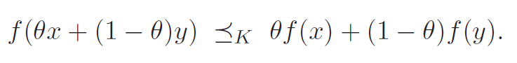
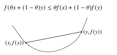
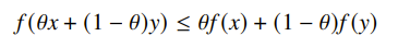
A function is convex if the domain is a convex set and for all $x, y \in dom f$ and $\theta \in [0, 1]$, we have

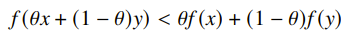
$f$ is concave if $-f$ is convex, and $f$ is strictly convex if

If you have equality, your function is affine, which means that it is both convex and concave.

Note: you shouldn’t interpret concavity as not convex (like what we did in convex sets). Many functions are neither concave nor convex; concave and convex share many of the same properties, just inverted.

Extended value extension

If $f$ is convex, the extended-value extension $\tilde{f}$ is defined as

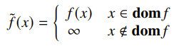
and this preserves convexity. It also simplifies notation, because if $\tilde{f}$ is convex, it means that the domain is convex and the original $f$ is convex. So we generally tend to use this.

• if we are out of domain, this infinity helps us keep the definition of convexity

• WE replace with negative infinity for concave functions

Examples

These are the most common or the ones that you can’t achieve easily through composition analysis

Both

• affine: $Ax + b$, or if you’re in matrix land, $tr(A^TX) + b = \sum_{ij} A_{ij}X_{ij} + b$.

• affine: $x^TPx$ in $P$, if you look at the summation definition

Convex

• The obvious ones: exponential, powers with exponent $\geq 1, \leq 0$, powers of absolute value

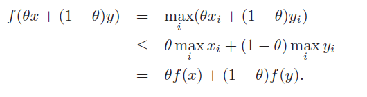
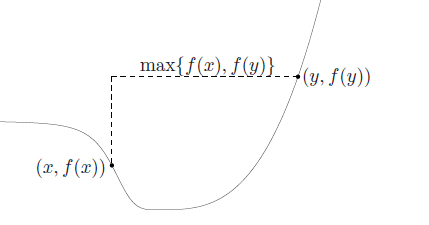
• Maxes $\max(x_1, …, x_n)$
  • Proof

    

• Any norms

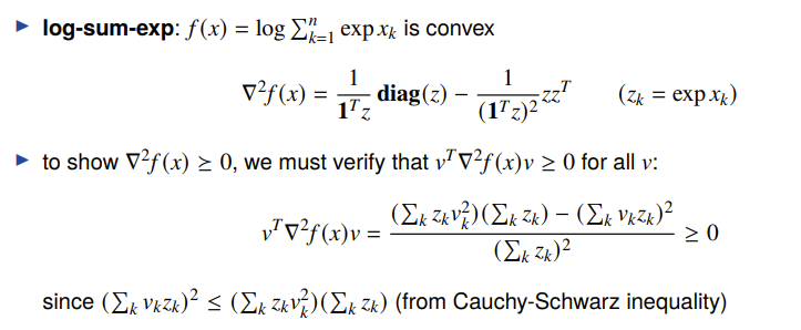
• log-sum-exp
  • Proof

    

• spectral norm (maximum singular value)

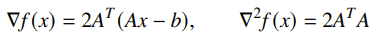
• least-squares objective
  • Proof

    

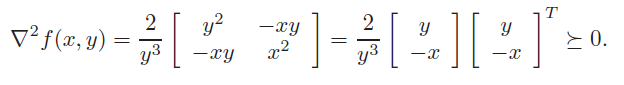
• quadratic-over-linear $x^2/y$ when $y>0$.
  • Proof

    

• quadratic with a PSD matrix

• $x \log x$ (negative entropy)

• Any sum of $k$ largest entries

• Proof

  Make the set of all $k$ entries in a set (should be $\binom{|S|}{k}$ of them. Take the sum (affine), and take the maximum (convex).

Concave

• The obvious ones: powers with exponent $\in [0, 1]$, logarithm

• Entropy

• Negative part

• Log-determinant
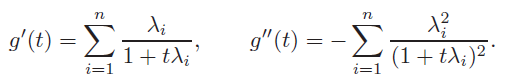
  • Proof

    

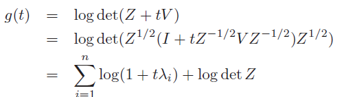
    where the eigenvalues are of $Z^{1/2}VZ^{-1/2}$. The derivatives are

    

• geometric mean

Alternate Definitions

These definitions are necessary and sufficient, so you can use them both ways.

Line definition

$f$ is convex if and only if $g(t) = f(x + tv)$ is convex in $t$ for any $x, v$. This is powerful because we can check convexity of arbitrary functions by looking at just one variable

First Order Condition

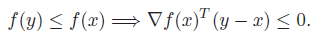
If the function is differentiable, we can use the first-order condition that says that $f$ is convex if and only if

Which just means that the first-order taylor expansion is a lower bound, or a global understimator.

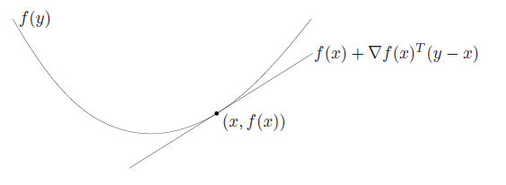
You can interpret this first-order approximation as the supporting hyperplane of the epigraph of $f(y)$.

Second Order Condition

We can also use the second-order condition that states that $\nabla^2 f(x) \succeq 0$. Strict convexity is $\nabla^2 f(x)\succ 0$.

Epigraph, sublevel set

Sublevel sets

An $\alpha$-sublevel set is defined as

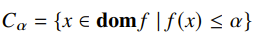
Sublevel sets of a convex function are convex by definition of convexity. However, the converse may not be true. Even if all sublevel sets are convex, the function may not be convex.

If $f$ is concave, the $\alpha$-superlevel set ($f(x) \geq \alpha$) could be helpful.

Epigraph

We can use the sublevel set to construct the epigraph of a function. This is defined as

You can imagine $t$ as the vertical sweep. You start filling when $t > f(x)$, which is exactly the shaded space above the graph.

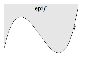
$f$ is convex if and only if $epi f$ is a convex set. So it is a very helpful tip to go between convex sets and convex functions.

Jensen’s and other inequalities

Jensen’s inequality 🚀

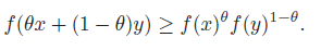
Jensen’s inequality arises from the definition of convexity

However, you can imagine building up this inequality inductively.

It works for any convex combination, even infinite ones like expectations.

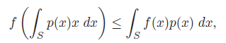
which gives us the final form with the expectation

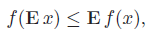
One interesting upshot: adding a zero-mean random vector to a convex function will make it worse: $E[f(x + z)]\geq f(E[x + z]) = f(x)$.

Deriving other inequalities

It turns out that many different inequalities can be derived from Jensen’s inequality.

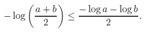
Arithmetic-geometric mean inequality:

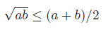
• Proof

  Use the equation below and take the exponential of both sides

  

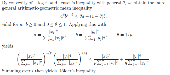
Holder’s inequality

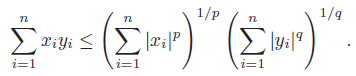
• Proof

  Use a general arithmetic-geometric mean inequality and plug some stuff in

  

Operations that Preserve Convexity

Sums

Non-negative weighted sums of functions will preserve convexity. A special case are just normal sums, infinite sums, and integrals. Concavity is also preserved through sums.

Affines

Convexity is also preserved if you precompose with an affine function, i.e. $f(Ax + b)$ is convex if $f$ is convex. You’ll see this format pretty often.

Adding or subtracting affine functions will preserve convexity or concavity. Multiplying an affine function may not. Same with dividing. Classic example: $f(x) = x^2, g(x) = x$, but $f*g$ is neither convex nor concave.

Maxes and Supremum

Pointwise maximums preserve convexity as long as $f_1, …, f_m$ is convex. And if you had something like $f(x, y)$, if $x$ is convex for all $y$, then $\sup_y f(x, y)$ is convex.

You can intepret maxes and supremums as the intersection of epigraphs.

Sidenote: concavity is preserved through pointwise minimums.

Second sidenote: these rules are also true for affine functions: pointwise minimums makes concave, pointwise maximum makes convex

Some forms of minimization

If we have a convex set $C$, the partial minimization $\inf_{y\in C} f(x, y)$ is convex. If you do partial maximization of a concave function, it is concave.

• Proof (Jensens’ inequality)

  The key trick here is using a bit of a tricky infimum definition with the $\epsilon$.

  

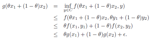
Visually, this looks like projecting $f(x, y)$ onto the $x$ space. If we think about things in terms of epigraphs, this is also a projection. The projection does preserve convex sets.

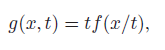
Function Perspective

The perspective of a function (very similar to the perspective of a convex set) preserves convexity

• Proof (epigraph)

  We create a mapping between epigraphs

  

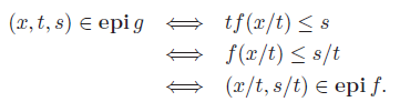
  And because the epigraph of $f$ is convex, so is $g$.

This is useful when you have cases where you have a function quotient which typically isn’t convex. But if you can massage something outside, then it can work.

Composition with Scalars

If you had $g:R^n → R$ and $h: R→R$, then $f = h\circ g$ is convex if

• $g$ convex, $h$ convex, $\tilde{h}$ nondecreasing

• $g$ concave, $h$ convex, $\tilde{h}$ non-increasing

Alternatively, $f$ is concave if

• $g$ concave, $h$ concave, $\tilde{h}$ nondecreasing

• $g$ convex, $h$ concave, $\tilde{h}$ non-increasing

The proof is very simple. Just differentiate $f$ twice

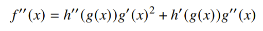
There’s a technicality with the extended-value extension. Remember that the extension pushes everything to infinity outside of the domain. So some functions that are non-decreasing in the domain are actually not non-decreasing with the extension. A good example is $x^2$ on $R_+$. It is non-decreasing, but once you do the extension, it is no longer non-decreasing because $f(x) = \infty$ when $x < 0$.

Commonly, this $h$ is some simple function like log and reciprocal.

General Composition Rule

The scalar composition rule is actually a special case of a more general truth about convexity. We derive laws from this expansion

Let’s suppose we have $g: R^n →R^k$ and $h: R^k → R$. Then $f = h\circ g$ is convex if $h$ is convex and for each $i$ in $h$, one of the following holds:

• $g_i$ is convex and $\tilde{h}$ is non-decreasing in $i$th argument

• $g_i$ is concave, $\tilde{h}$ non-increasing in $i$th argument

• $g_i$ is affine

For concavity, if $h$ is concave and for each $i$ in h, we get concavity if

• $g_i$ is concave and $\tilde{h}$ is non-decreasing in $i$th argument

• $g_i$ is convex, $\tilde{h}$ non-increasing in $i$th argument

• $g_i$ is affine

Common forms

• $h(x, y) = xy$: COMMON MISTAKE! THIS IS AFFINE, and we can’t say much about it. Counterexample: $\log(x), x$.

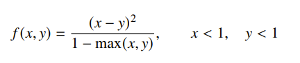
• $h(x, y) = x^2/y$ for $x > 0$: convex in x, y

• $h(x, y) = \sqrt{xy}$ is geometric mean and therefore concave

Constructive Convexity Analysis

This is a general method that is really useful. You start building up the function from the inside out. You consider each operation iteratively. Here are some quick tips

• addition: if you add affine to anything, you preserve that property. Convex + convex = convex,

• When you compose a function, it might have different (very different) impacts on the sign, derivative, and convexity. Convex rules are typically harder.
  • sometimes convexity doesn’t care about the derivative

• Quad over lin: can give special case of reciprocal (doesn’t depend on first derivative)

• Alternate idea: parse tree

  This is a general method that is super, super useful. You build a parse tree

  • leaves are either constants or base functions.

  • Nodes are elementary operations

  • Edges are compositions

  With each step, indicate the sign and the curvature. These two properties can be derived from elementary operations.

  • Example

    If we consider the function

    

    We can build up this tree

    

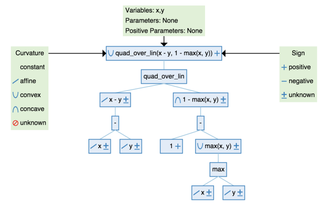
This constructive process is used in disciplined convex programming, which is how convex functions are build from their atomic constituents.

It is important to note that the constructive decomposition is sufficient for convexity, but it is not necessary.

Conjugate Function

We define the conjugate of a function as

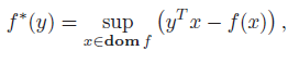
This might seem really weird, but immediately we can see that this is the supremum of an affine function, meaning that $f^*$ is convex, regardless of what $f$ is. The domain includes any $y$ such that the supremum yields a finite number.

Examples

• $f(x) = ax + b$, so $yx - ax + b$ is only value of $y = a$, so the domain is $\{a\}$ and $f^*(a) = b$.

• Exponential $f(x) = e^x$ has $xy - e^x$ as unbounded if $y< 0$. Otherwise, you can derive that pointwise maximum is $x = \log y$, meaning that $f^*(y) = y\log y - y$.

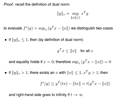
• The conjugate of the norm $||z||^*$ is defined as $0$ if $||z||_* \leq 1$ and $\infty$ if $||z||_*> 1$, where $||z||_* = \sup_{||x||\leq 1}x^Tz$ is the cdual norm. If you think about this for a second, it should make sense

• Proof

  

Basic Properties

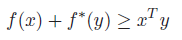
The Fenchel's inequality follows directly from the definition of the conjugate:

The conjugate of a conjugate function is the original function (it’s not obvious) $f^{**} = f$.

• Proof (TODO)

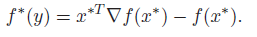
If $f$ is differentiable, the conjugation is also called the Legendre transform. If you take the derivative WRT x, you’ll get that it equals $y - \nabla f(x)$, which means that the conjugation finds the $x^*$ such that $y = \nabla f(x^*)$, which makes the conjugate function

Quasiconvex functions

A function is quasiconvex or unimodal if all sublevel sets are convex. Recall that when we talked about sublevel sets, we mentioned that convex function have convex sublevel sets but not the converse. This is the converse situation.

A function is quasiconcave if every superlevel set is convex. Functions that are both quasiconvex and quasiconcave are quasilinear (but some of these functions are very far from being actually linear!).

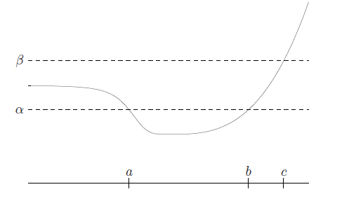
You can see in the diagram above that this function is indeed not convex, but the sublevel sets are convex.

Intuitively, quasiconvex functions must only have one minimum. If there are two minimums, imagine slicing the function right above the two minimums. You’ll get two disjoint sets that are definitely not convex.

Proof tips

Use the first order or second order definitions, as well as the sublevel set definition. The sublevel set definition is often easier, because you just have to show that the set is concave. You can also express it as a family of convex functions $\phi_t(x) \leq t$.

Jensen’s Inequality for Quasiconvex

A necessary and sufficient property for quasiconvexity is this:

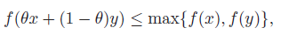
Which essentially means that there isn’t a hump somewhere in the middle (and this enforces the unimodal constraint)

Like convexity, it is sufficient to check this property on lines.

In real numbers

If a function operates on real numbers, it is necessarily and sufficiently quasiconvex if it is non-decreasing, non-increasing, or it changes direction only once.

First Order Condition

The first order condition is as follows:

which essentially means that if a point is below, then the path approaching this point must be going in one direction. Geometrically, it means that $\nabla f((x)$ is the supporting hyperplane to the sublevel set $f(y) < f(x)$.

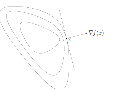
Note that this doesn’t constrain $\nabla f(x)$ to be non-zero outside of a minimum point. In fact, the constraint allows $\nabla f(x)$ to be zero anywhere.

Second Order Condition

The second order condition is as follows: if $f$ is quasiconvex, then for all $x$ in domain and $y \in R^n$, we have

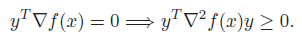
Thsi means that if $\nabla f(x) = 0$, then $\nabla^2 f(x) \succeq 0$ (PSD). If $\nabla f(x)\neq 0$, then $\nabla^2 f(x)$ must be PSD on the subspace $\nabla f(x)^\perp$. This implies that there can only be one negative eigenvalue.

The converse is also true: if the conditions are satisfied, then $f$ is quasiconvex.

Operations that preserve quasiconvexity

There are some overlaps with operations that preserve convexity

• non-negative weighted maximum

• pointwise supremum

• Composition with affine or linear-fractional transformation

• Minimization $g(x) = \inf f(x, y)$

Log-Concavity / Log Convexity

A function is log-concave if $f(x) > 0$ and $\log f$ is concave. Vice versa. From this derivation, we konw that $f$ is log convex if and only if $1/f$ is log concave.

Mathematically, this just means that the following property is true:

A log-convex function is convex, because by composition rules, $e^h$ is convex if $h$ is convex. However, not all convex functions are log-convex.

Proof tips

• Log concavity and log convexity are related through reciprocals. Sometimes it’s easier to work with the reciprocal of a function

Examples

Affine function, powers, exponential, CDF of gaussian, gamma function, determinant.

Properties

We can look at the second derivative of the log function

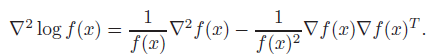
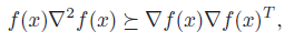
which will lead us to conclude that $f$ is log-convex if and only if

Log-convexity is preserved under multiplication and positive scaling. The sum of log-convex functions is also log-convex because of the composition rule

This is also true for weighted sums and integrals.

Log-convexity is still preserved under maximization because log is monotone increasing, and the maxes commute with the logs

Convexity with general inequalities

Previously, we have been using special versions of inequalities. Now, let’s look at what happens when we have a generalized inequality? This is helpful because sometimes the inputs don’t necessarily have a strict ordering. This allows us to generalize convexity to functions that are not necessarily scalar outputs.

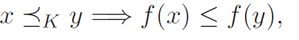
Monotonicity

If we have some metric $K$, then we call the function $k$-nondecreasing if

We can also write monotonicity in the first order, using the restriction

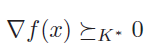
Note: this is tricky—this is related to the dual inequality, which we didn’t cover extensively. But just know that you need the dual cone of $K$ to get the first order

Moving to convexity

As such, we can arrive at the convexity definition, for some function $f:R^n → R^m$