Tips and tricks

• Probability distribuiton: add a constraint $1^Tx = 1$

Notes on norms

Least squares objective is minimizing the sum of squares, not the L2 norm which has a square root. The L2 norm, or any sort of p-norm is “linear” in each component because you raise the component to $p$, sum, and then take the $1/p$ power.

Norm Approximation

The big objective is to minimize $||Ax - b||$, where $A \in R^{m\times n}$ and $m\geq n$. This norm could be any valid norm.

Ways of interpreting

• Approximation: Get $Ax^*$ to be the best approximation of $b$

• Geometric: $Ax^*$ is the point closest to $b$ in the norm

• Estimation: get a linear model that matches the observed data as close as possible

• Optimal design: $Ax$ is the resutl, $x^*$ is the best design for some constraint

Variants

• Euclidian approximation: closed form solution

• Squared euclidian approximation: also closed-form solution because you can write the squared norm as $f^Tf$.

• Chebyshev / minimax approximation: solved through LP

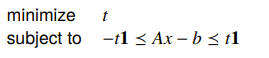
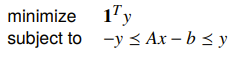
• L1 norm: solved through LP

Penalty Approximation

This big objective is to minimize $\phi(r_1) + … + \phi(r_m)$ subject to $r = Ax - b$. Here, $\phi$ is a scalar, convex penalty function.

Common examples

• Quadratic

• Deadzone linear $\phi(u) = \max\{0, |u| - a\}$

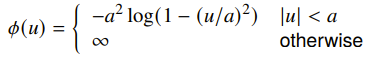
• Log-barrier

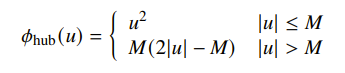
• Huber (linear growth for large $u$ makes it robust to outliners)

These different penalty functions can yield quite different losses. Most notably, an absolute value cost typically yields a sparse solution.

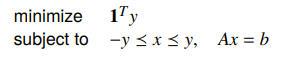
Least-Norm problems

This is when you minimize $||x||$ such that $Ax = b$. There are a few interpretations

• Smallest point in the solution set of $Ax = b$

• Estimation: if $b = Ax$ are perfect measurements of $x$ and the norm is the implausibility, then $x^*$ is the most plausible given the constraints

• Design: if the norm is something related to efficiency, then $x^*$ is the most efficient

Variants

• least euclidian norm

• Least sum of absolute values: solve this through LP

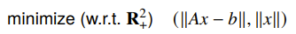
Regularized Approximation

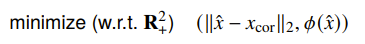
Regularized approximation is a bi-objective problem where you want to reduce the quantities of two things

Common interpretations

• estimation: you want to fit something under the prior that it is small

• optimal design: $x$ is expensive, so you want to have a cheap solution

• robust approximation: smaller $x$ is less sensitive to errors, so you want to minimize this

Variants

You typically scalarize the problem to get $||Ax - b|| + \gamma ||x||$, and this traces the optimal tradeoff curve (see notes on Pareto optimality)

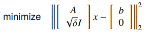
• If we have L2 norm, we call this Tikhonov regularization or ridge regression, and it has a least-squares solution

You can also have a linear dynamical system defined as

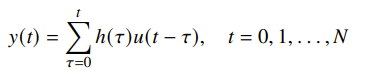
This particular setup is useful if you want to shape the impulse response of a function. More precisely, you want to optimize $u$ over three properties: you want to reduce the estimation error, minimize input magnitude (the norm of $u$) and you want to reduce variation of the input (the difference between $u(t)$ and $u(t+1)$ should be small). Once you scalarize, this problem is a regularized least-squares problem becuase all of the things can be expressed as sums of squares.

You can also just try to fit a signal directly, using different variatns of the regularizer that cares about how the $\hat{x}$ changes through time.

• Quadratic regularizer can remove noise, but it acts like a lowpass filter so it can’t do sharp edges

• Absolute value (L1) regularizer can keep the sharp curves

• Huber regularizer is robust to outliers

Robust Approximation

The big objective here is to minimize $||Ax - b||$ but the $A$ is uncertain. Under these conditions, there are two philosphies:

• stochastic: assume $A$ is random, minimize the expectation

• worst-case: minimize $\sup_{A \in \mathcal{A}}||Ax - b||$

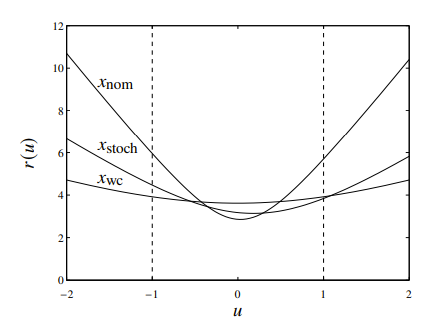
Examples

If $A(u) = A_0 + uA_1$ where $u \in [-1, 1]$, then you can compute both the stochastic and the worst-case. In general, they both perform pretty well. The plot shows $r(u) = ||A(u)x - b||_2$.

The stochastic robust least-squares setup is where we have $A = \bar{A} + U$, where $E[U] = 0, E[U^TU] = P$ for some matrix. We want to solve the stochastic least-squares problem, and it turns out that if you do your algebra out, you get

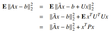
Which is essentially a strategically regularized least squares problem. If your $P$ is a scaled identity matrix, then this is just ridge regression.