Key things to know

In hard-SVM, we assume that things are separable. We want to find the best line that separates things

We predict things by

to optimize $w, b$, we use the following objective:

After lagrangian hardship, you get that the optimal solution has the form

which means that the kernel trick can be used

If we are doing soft-SVM, we can think of SVM as minimizing hinge loss + L2 regularization

The big idea

Given two clusters of data, how can we separate it such that the margin between the two clusters is as big as possible?

In the notes below, we will mostly talk about linear SVM's. But then we'll talk about how we can use a kernel to do an arbitrary boundary with this "linear" classifier!

Notation

Previously in logistic regression we used labels $y \in \{0, 1\}$. Now, we will use labels $y \in \{-1, 1\}$, and we parameterize the model as

This also means that we drop the convention that $x_0 = 1$.

Furthermore, $g$ is no longer a continuous function. Rather, if $w^T x + b < 0$, it predicts $-1$, and if it's $\geq 0$, it predicts $1$. We call $g$ as a $\text{sign}$ function

So a trained SVM model is just like a kernelized perceptron

What is a margin?

Back in logistic regression, you could understand $g(\theta^T x)$ as a measure of model confidence that $x$ is a positive example. If it's greater than 0.5, we just called it a positive prediction, and vice versa.

The further we are from that dividing line of $\theta^T x = 0$, the more confident we are. This length is called a margin.

Functional margins

The functional margin of $(w, b)$ with respect to a training example is defined as

As you notice, if $\gamma$ is positive, then we are classifiying correctly. The larger the $\gamma$, the more confident we are.

Functional margins WRT a set

Given a training set $S$, we define the functional margin of $(w, b)$ with respect to $S$ as

or, in other words, the least confident (or the most incorrect) prediction. This is the definition we use when we talk about functional margins.

Geometric Margins

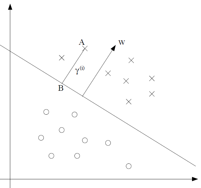
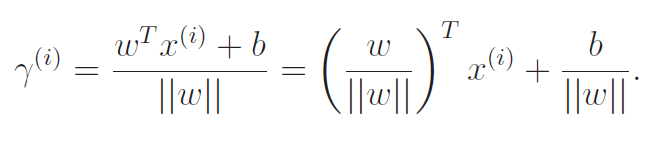
We provide another way of understanding a margin. This time, geometrically. Above, we see a margin $w^Tx + b = 0$ and the distance from points. We know that $w / ||w||$ is the unit vector. As such, we can imagine moving back from a point A by traveling length $\gamma$ to point B. This is mathematically expressed as

When we solve for $\gamma$, we get

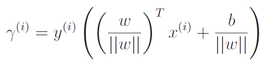
Now, margins must be positive. To account for negative distance, we multiply everything by $y$.

Relating geometric and functional margins

Note how the geometric and the functional margins look very similar, and they are equivalent if $||w|| = 1$.

The geometric margin value does not change with a scaling of $w$ and $b$ because we divide by the weight norm. A good margin quantifier exploits this feature because scaling $w, b$ does not change the line at all. Therefore, the margin shouldn't change.

Optimal margin classifier objective

The direct objective

What do we want to optimize? We want to maximize the margin of a training set, which means maximizing the lower bound of $y(w^Tx + b)$. This looks like

Writing this direct objective

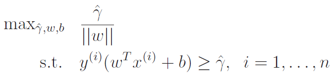
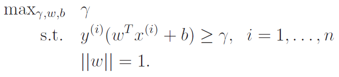
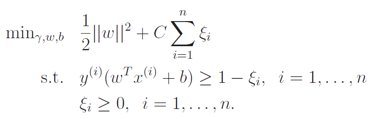
With this goal in mind, we start to formulate the constrained optimization problem. Our overall objective is

but we constrain it to $||w|| = 1$ to keep the functional margin and the geometric margin equivalent.

In addition, we turn the inner $\min$ into another constrain, to get us this objective.

However, we reach a problem. Our constraints are not affine, which means that we can't apply the dual legrangian properties (see lagrange section) to our problem. Duality allows for an easier pathway of optimization.

Improving the objective

The problem child is the $||w||$ in the way. We motivated it due to equivalence between margin types, but can we just compute $\gamma_{func}$ and convert it to the geometric? This is our motivation below:

Unfortunately, this is still not there yet. Our constraints are linear, but the objective is not convex. the KTT conditions are not met yet.

The final form

Now, to make the final push, we make one crucial insight. The margin is a unitless constant, and we are dealing with the functional margin, which is not invariant to scaling. So what if we just defined some scalar $c$ such that $c = 1 / \hat{\gamma}$? In this case, we would have $y(cw^Tx + cb) \geq 1$. And we can swallow this $c$ into the $w$ and the $b$.

Essentially, we argue that instead of maximizing both the $\hat{\gamma}, ||w||$ as we were trying above, why don't we hold one thing constant? After all, this $\gamma$ and the $w$ are related, SPECIFICALLY because we are dealing with the FUNCTIONAL margin.

With this insight, we reframe the objective to be $\max_{w, b} 1 / ||w||$. To maximize this, all we need to to is minimize $||w||$, or $||w||^2$. We arrive upon this objective :

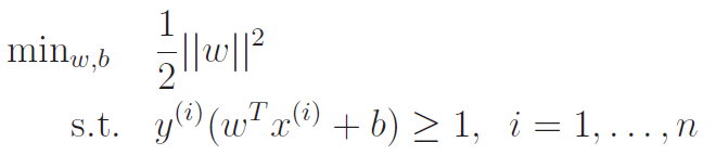
Now this is what we are looking for! A convex function with a linear constraint. The solution set $(w, b)$ gives the optimal margin classifier, and this can be solved using quadratic programming.

Optimal margin classifier derivation

Understanding the role of $\alpha$

Now, we are ready to start using Lagrangians to derive the optimal margin classifier. We need the general lagrangian. First, we define the constraint function $g_i$:

• quick refresher on KTT conditions

  

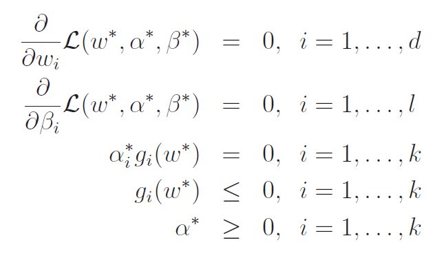
We will eventually multiply $g_i$ by its lagrange constant $\alpha_i$.

Now, let's look back on the KTT conditions (see lagrangians notes). Recall that we have $\alpha^* g(w^*) = 0$, meaning $\alpha > 0$ only when $g_i(w) = 0$. This happens only with the margins that are the closest. If you're confused, refer back to our objective. It's the lower bound for the margins.

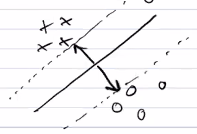
We represent this graphically below.

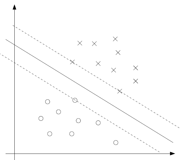
The solid line is the boundary, and the maximum margin is denoted with the dotted lines passing through the points with the least margin. These points are the ONLY points whose $\alpha > 0$. We call these points the support vectors, and we note that only a small subset of the dataset are support vectors.

Intuitively, it means that anything that isn't a support vector can essentially be removed from the dataset without changing ANYTHING. We will see the math behind this in a second

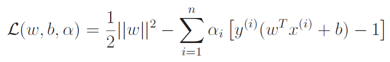
The Lagrangian

The Lagrangian becomes

Usually, we want to find min-max. However, this lagrange problem satisfy KTT because we satisfy PSD and the constraint is affine.

As such, we can also find the max-min. This means that we first minimize $\mathcal{L}$ with respect to $w, b$. Then, we maximize that expression with respect to $\alpha$.

Minimizing

We just take the derivative and set that equal to zero. First, let's start with $w$.

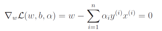
This means that

And now, let's do $b$.

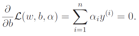
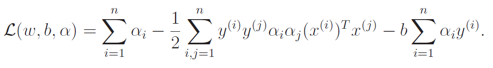
We didn't solve for $b$, but we arrived at a constraint. Now, let's take these two insights and simplify the lagrangian. Here are the steps we took: (the original is reproduced below for clarity)

1. simplify $||w||^2$ using $w^Tw$. We can directly do the transpose on the summation because transpose distributes.

2. Simply $w^Tx$ using the same technique

3. Note that $\frac{1}{2} ||w||^2$ has the exact same form as $\alpha_iy^{(i)}w^Tx^{(i)}$, so we combine them into the middle term below. (1/2 - 1 = -1/2 is where that negative comes from)

4. the first and last terms below are from the other parts of the second term of the lagrangian.

We arrive at this form:

We also notice that the last term we derived to be $0$. Therefore

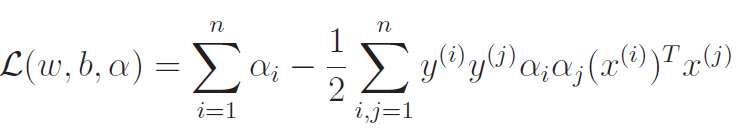
As such, we have completed the min step of the optimization. Now, let's to the max!

Maximizing

Now, this expression above is what happened after we perform a minimization. Now, with these constraints in mind, we will maximize the expression above WRT $\alpha$ with two key constraints shown below

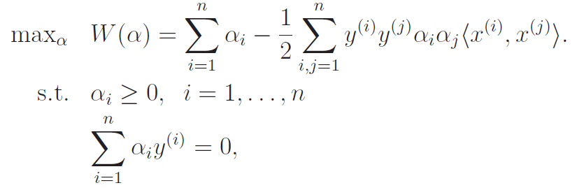
The first constraint arises from the definition of $\alpha$, and the second constraint arises from our derivation of $b$. Now, the implicit third constraint lies in how we wrote the maximization objective. We didn't use $w$, but rather, the expression we had above.

How do we do this?? Well, let's talk about it in SMO (scroll down). For the next few sections, we assume that we can have this solution and we'll talk a little bit about what we can do about it.

Deriving the needed $w, b$

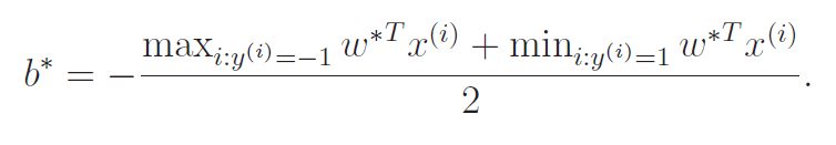
Once we solve the $\alpha$, we will be able to find the $w$ through the equation below.

Now, the $b^*$ can be derived. How? Well, it has a graphical intuition

With our $w^*$, we've already settled on an angle of the line. We know our final solution has the form $w^Tx + b$. We want to find the closest points (the support vectors) and then just take the average of those points.

• $b_{-1} = -\max_{y = -1} (w^*)^Tx$

• $b_{1} = -\min_{y = 1} (w^*)^Tx$

Now, the center is just the average:

The Support Vector Insight

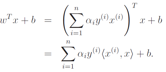
But this allows us to do something very interesting. When we run the model, we just need to do $w^Tx + b$. We can replace the $w$ with the $w^*$ definition, which gets us the following:

Now, this gives us a lot of interesting insight. So if we've found the necessary $\alpha$, then predicting the output is equivalent to taking the inner product with all the points in the training set. And this is even neater: as we recalled, $\alpha$ is only non-zero when $x^{(i)}$ is on the edge of the margin! So, the prediction can be done by just looking at a select few points, which we called support vectors. Nice!!

The Kernel Insight

We note that at test time, we get that

Hold up! This inner product is reminiscent of the kernel! So...how can we extend this linear classifier derivation to arbitrary boundaries?

So this is how it works at test time, but what about training?

Well, recall that our maximization step looks like this

So you see the inner product? This is the kernel corresponding to the identity feature map. In reality, we can replace this kernel with anything! This gets us

And there we have it! We are suddenly able to create an arbitrary boundary that is more complicated than a linear boundary!

The infinite kernel: arbitrary boundaries

Recall that we have the gaussian kernel

What if $\sigma$ approached $0$? Recall that our prediction algorithm is

as such, the value of the summation is determined almost solely by the point $x^{(i)}$ that is the closest to $x$ (let's assume that $\alpha_i = 1$ for simplicity.) This means that we can draw a perfect boundary between two classes scattered arbitraily!

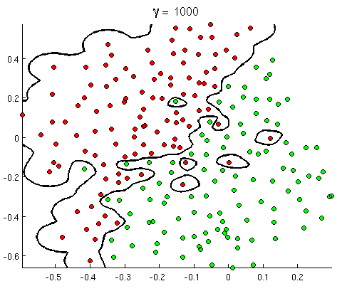
This goes back to the idea that the gaussian kernel is infinite dimensional. It can make any boundary it wants! It also goes to show that the smaller the $\sigma$, the more "overfit" your boundary can become.

Regularization (soft SVM)

If $x$ is linearly separable, then the previous derivation of SVM is good enough. However, real data is not that optimal. It may not be linearly separable, or an outlier might require a very severe margin

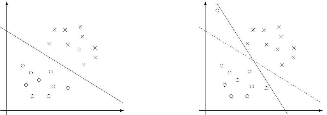
(when we add one outlier point, the margin must pivot to a very extreme angle).

Kernels may help when we are dealing with non linear separable data, but for outliers, we can use a regularizer ($\ell_2$ regularization).

Essentially, we allow things to have narrower margins (including negative margins meaning an incorrect prediction) but we want to minimize the amount of "borrowing" we have to do, which is what we do in the $\min$ expression. The legrangian is formulated as follows:

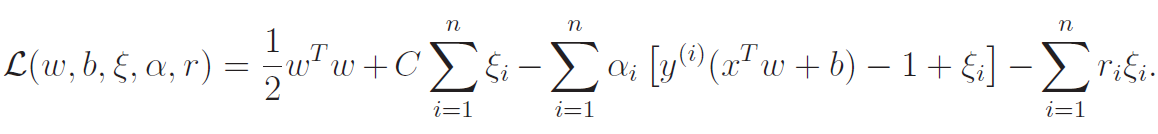
Here, $r, \alpha$ are our lagrangian multipliers. After doing the optimization and simplifying, we get the following sub-objective

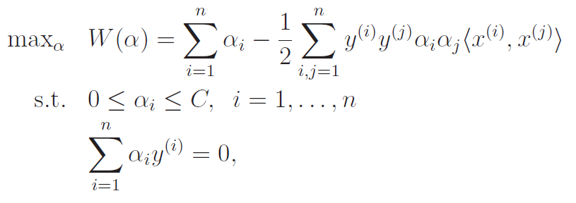
Interestingly, the only change to the dual problem is that the $\alpha_i$ is bounded by another constant $C$, which makes sense because we're using an l2 regularizer.

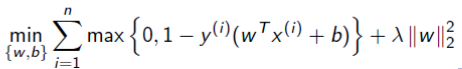
Soft-SVM as hinge loss

We can actually rewrite the lagrangian as a sort of hinge loss. Essentially, instead of setting a lower bound on the borrowing, why don't we just minimize the borrowing directly?

Here, we arrive at the Hinge loss. When a model is accurate, the $y$ and the $w^Tx + b$ will have the same sign and therefore yield zero or close to zero losses.

SMO Algorithm (solving the dual problem)

Now, in the case of SVM, after performing one round of Lagrangian optimization, we arrive at another constrained optimization problem. One example is below:

How do you actually solve this?

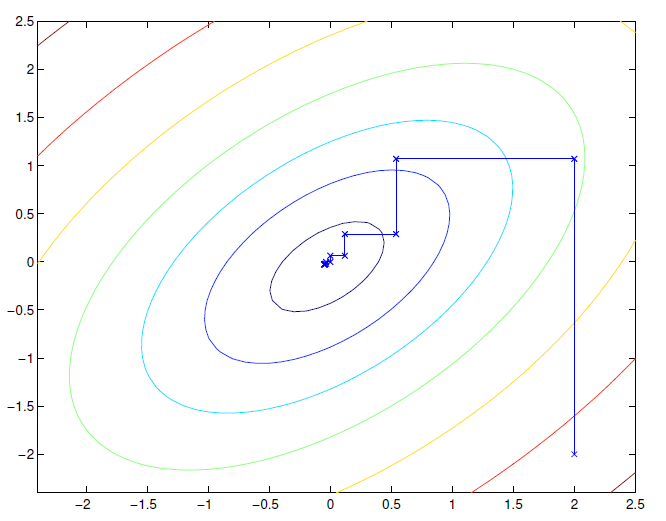
We can use a technique called sequential minimal optimization, which does something interesting. It optimizes one parameter at a time. So it might tine $\alpha_1$, and then tune $\alpha_2$, and so on.

This is what it might look like:

Adapting SMO to work with our problem

The issue is that we can't just tune one $\alpha_i$ at a time, because $\sum \alpha_i y = 0$. As such, we must perform SMO with a pair of $\alpha$.

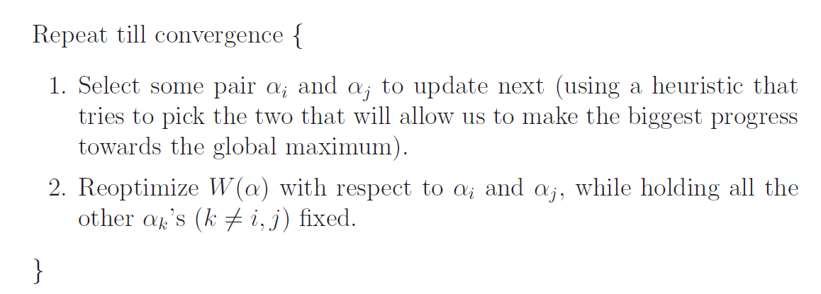
Let's say that we picked $\alpha_1, \alpha_2$. This optimization problem is actually really easy, because $\alpha_1y^{(1)} + \alpha_2y^{(2)} = -\sum_{k \neq 1, 2} \alpha_k y^{(k)}$. This is just a line! Furthermore, in the case of the regularized SVM, we also know that $\alpha \leq C$, so we are just confined to a short line segment.

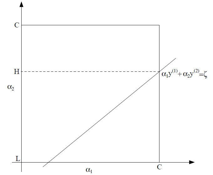
Because $y \in \{-1, 1\}$, we can actually write $\alpha_1$ in terms of $\alpha_2$ as

The objective then becomes

If you look at the definitino of $W$, this just means that $W$ is a quadratic function in $\alpha_2$, which has a guaranteed extrema. In this case, it's a maximum.

To check for convergence, we just verify that the KKT conditions satisfied within some error margin.

SVM vs Logistic regression

There's a really subtle difference here that is very important. Logistic regression does NOT assume that there is a direct boundary between the data. As such, it will find a $\theta$ that creates enough "fuzzy zone" to best represent the data.

However, SVM's without regularization assume that there IS indeed a direct boundary between the data.

If you are sure that the data is separable, you should use an SVM. This is because if you used a logistic regression, the $\theta$ will diverge as it makes the boundary sharper and sharper. If we start with an infinitely sharp boundary with the SVM, there's no need for this weird behavior.