From factor analysis

Factor analysis learned a matrix $\Lambda$ that effectively turned a low dimensional representation $z$ into high-dimensional $x$ space. It used the EM algorithm to get the encoding. As it turns out, if we only care about low-dimensional representation, we can also use principal component analysis (PCA), which only uses eigenvectors

Often, your different dimensions can be highly correlated. For example, you might have miles per hour and kilometers per hour. In reality, you only get one piece of information. We can extract this through PCA!

PCA can work as noise reduction, overfitting reduction, and can even help us visualize high-dimensional data.

Dimensionality reduction

Here's the big idea. How can we project a set of points $x$ with dimension $d$ onto a subspace of dimension $k$ while maintaining as much information as possible? In other words, if $A$ were the projection matrix and $z = Ax$, then we want $\hat x = A^{-1}z$ to be as close to $x$ as possible.

The derivation

Projections

When we talk about projection matrix, we just want to project some space onto an orthonormal basis $u_1, ..., u_k$, the vectors of which make up $A$. We need to find these vectors!

We establish some $\bar x$ which we subtract from $x$ before projecting. This is just so our later derivation works out perfectly; it does not influence the conceptual understanding of the problem. To project, we just do

Now, $z_i$ would be in the changed basis, and $x, u_i$ would both be WRT the canonical basis. Here's the tricky part: we can imagine that we have $d$ orthonormal vectors such that we are just projecting onto a rotated coordinate without losing any information. However, when we do compression, we only pick $k$ of these (and we order $u_1, ... u_k$ to be the most important, somehow)

We can express $\hat x$ as the following:

Think about this for a second—it's important

Cost function

Our error as as follows:

Let's make sure that we digested that correctly: so the first part inside the squared is another way of representing $x^i$, and the second part inside the squared is what we had above

We note that the two sums can partially cancel and we get

Now, this squared error is actually a dot product. So, we can write this out by splitting into cross terms and non-cross terms

Now, we recall that $u$ is an orthonormal basis. As such, the second term just cancels out, and the first term simplifies

So, tl;dr—to minimize the error, we just need to minimize the coefficients OUTSIDE of our selected basis. This makes a lot of sense!

The covariance matrix

But how do we minimize this? Well, let's expand what we know about $z$

Let's rewrite and move the summations around

We did this because $(y^Tz)^2 = y^Tzz^Ty$ .

And if we assign $\bar x = E[X]$ or the mean of the $x$, then we have the following:

(recall that covariance is just $\frac{1}{N}\sum_i^N(x - E[X])(x - E[X])^T$)

So our error just becomes finding the minimum of a quadratic form!

Eigenvectors

Here's the rub: Why don't we just use the eigenvectors of $\Sigma$? We need to select some basis that minimizes our error, and any orthonormal basis is equivalent under one transformation. As such, we can pick what is most convenient.

If $u_j$ is an eigenvector with eigenvalue $\lambda_j$, then

(take a minute to convince yourself of this)

As such, to minimize the error, we simply need to pick $k$ eigenvectors to form $u_1, ... u_k$, and we pick it by selecting the eigenvectors of $\Sigma$ with the highest eigenvalues!

Algorithm, reviewed

1. start from an $N \times d$ matrix $X$

2. Subtract center mean from each row to form $X_C$

3. Compute covariance matrix of $\frac{1}{N}X_C^TX_C$ (take a second to convince yourself that this is indeed the covariance. It helps to consider matrix multiplication as a series of outer products.

4. Find the eigenvectors and eigenvalues of $\Sigma$, and the principle components are the $k$ eigenvectors with the highest eigenvalues. It's worth noting that the eigenvectors are the orthonormal basis, and they are in the canonical space (i.e. non-transformed space). Confused? See below for a practical example.

To compress a point, just compute the inner product with these normalized eigenvalues!

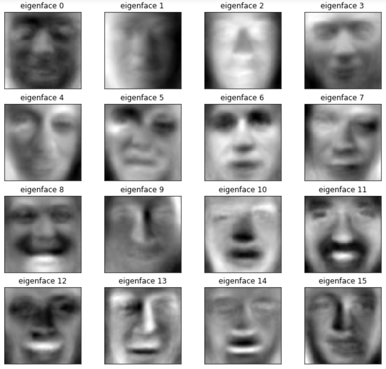
Eigenfaces

In eigenfaces, we had an $N\times d$ matrix where the $N$ are the number of people and the $d$ is a flattened version of the image. For example, if the picture were $100 \times 100$, then $d = 10000$.

By computing PCA on it and selecting only the $k$ top eigenvectors, we are able to generate eigenfaces, which are the eigenvectors corresponding to the k-top eigenvalues. Each eigenvector corresponds to a picture. We can reconstruct faces by projecting an image onto the eigenface basis. The larger the $k$, the better the reconstruction.

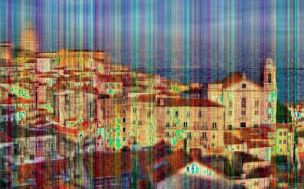
And here's an image of a city reconstructed from eigenvectors

SVD to speed things up

Essentially you write $X = WSV^T$, where $X$ is the data matrix (row per datapoint), $W$ is a weight matrix, $S$ is the singular value, diagonal matrix, and $V$ is the singular vector matrix.

You can think of $W$ as the coordinate of $x^i$ in eigenspace, and $S$ contains he eigenvalues $\lambda_j$.

SVD helps because you don't need to compute $\Sigma$ explicitly. Rather, you do some cool math (I'll figure this out later) and eventually get the $k$ eigenvectors that you desire.

Another key distinction is that SVD isn’t lossy. You’re just factorizing the matrix into three components. You drop components by zeroing out elements of $S$.

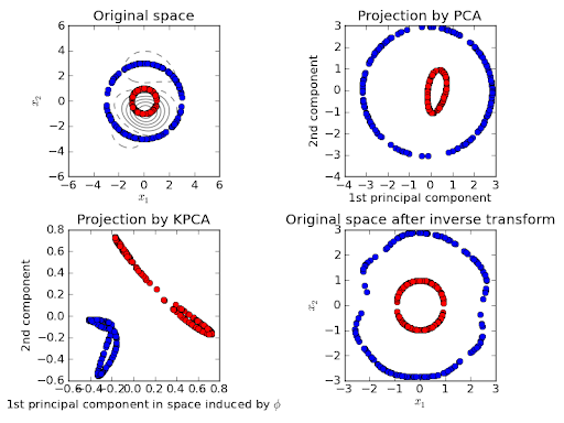
Kernel methods

You can also substitute the dot products we used with a kernel. Without getting into this too much (it's a similar idea), you can express far more complicated features with a kernel.