Naive Bayes

Previously, our $x$ was continuous. This allowed us to us GDA and other classifying methods. But what if each element of $x$ were discrete? This might be something like classifying a car based on various binary features, each encoded as an element in a vector.

Or, you might be representing an email through a sparse vector that has a 1 if the word is found, and a 0 if the word is not found. In this case the vector would the be the length of the english dictionary.

In the case of GDA, we essentially had to make a joint distribution $x | y$. However, this is infeasible with this high-dimensional vectors. If we wanted to figure out $p(x | y)$ of the dictionary example, it would be completely intractable. As such, we make one crucial and strong assumption: the $x$ is conditionally independent given $y$

In other words, if $y = 1$, then the outcome of $x_a$ does not influence $x_b$. Intuitively, it sort of makes sense. If you're making a spam detector, then certain words will just be more prevalent in spam, irrespective of what the other words are. So knowing that an email is spam or not spam is sufficient information to create a distribution.

This is known as the naive bayes assumption, and the resulting algorithm is the Naive Bayes Classifier. The formulation is below:

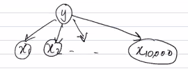
Graphically, we express the dependency relationship as

Fitting

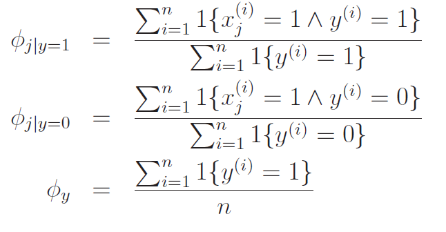
Let $\phi_{j | y = 1}$ be the $p(x_j = 1 | y = 1)$, and $\phi_{j | y = 0}$ be $p(x_j = 1 | y = 0)$. And let $\phi_y$ be $p(y = 1)$. If we do a maximum likelihood estimate, we get that

Intuitively, this all makes sense. We save these $\phi$ as the model parameters.

Predicting Naive Bayes

This is very simple! Just use Bayes rule to turn the generative model into a predictive model

Approximating continuous distributions

We can always model continuous distributions with Naive bayes; we just need to discretize the continuous values into bins. At times, if the data isn't distributed according to gaussian, a discretized Naive Bayes can do a better classifier.

Laplace Smoothing

The problem is that with sparse encodings, you might get the $p(x | y = 1) = p(x) = 0$, which results in an indeterminant form. In other words, if you haven't seen an example before, Naive Bayes will break.

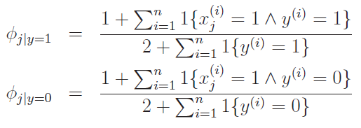
Laplace smoothing just assumes that you have one observed event for every output type. In other words, if $x$ takes on two values, we add 2 to the denominator and 1 to the numerator when computing $\phi$.

The intuition comes from the idea of having a prior, uniform distribution. In other words, before I see anything, I assume that all classes (x = 1, x = 0) are equally likely. This is why I add 1 to the top and 2 to the bottom.

When should I use naive bayes?

Naive bayes is quick and dirty and easily adaptable. It's a good first step, and it's a good sanity check.

Refining Naive Bayes (multinomial)

Let's focus on a spam classification algorithm, because it helps us frame a different version of naive bayes.

Naive Bayes relies on a distribution that doesn't care about word order. You can think about the naive process modeling generation as the following:

1. flip a weighted coin to see if we are sending a spam or non-spam email

2. For every word in the dictionary, flip its weighted coin (the probabilities depend on spam or no spam). Its presence or absence in the email depends on this coin result.

However, messages like bank loan bank have the same $p(y|x)$ as bank loan loan bank, which doesn't seem quite right.

This original form of Naive bayes is called a multivariate bernoulli event model, which means that there are many events (multivariate) but each event is a bernoulli outcome. In this context, $\phi_{j | y = 0} = p(x_j = 1 | y = 0)$ means "what is the probability that the $j$th word in the dictionary happens given that we are not sending spam?"

Looking at a multinomial

Why don't we start looking at the word generation, and less at the dictionary? In other words, can we model $x_j$ not as a bernoulli word presence, but as a distribution over all the words in the dictionary? In this context, $\phi_{k|y = 0} = p(x_j = k | y = 0)$ means "what is the probability that the $j$th word in the EMAIL happens to be the $k$th word in the dictionary?"

We call this a multinomial event model, in which there are many independent multinomial events. We can think of the generation process as the following:

1. flip a weighted coin to see if we are sending spam

2. for every word in the EMAIL, throw a (very large) weighted dice and write down the word that comes up.

Independence equations

For both version of naive bayes, we can use the equation

although they mean very different things. For the multivariate bernoulli, we are saying that the different variables are independent. For the multinomial event model, we are saying that the different word choice events are independent.

The dice vs coin analogy can be helpful.

MLE in the multinomial

We define the likelihood as the following:

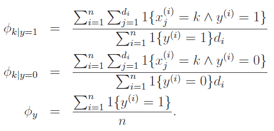
Notice how there's a double product: one for the word (constructive) and one for the dataset. By taking MLE , we get the following:

This makes intuitive sense. You are counting the number of conditional occurrences of this particular word, and you are dividing that by the total number of words ($d_i$).

Laplace smoothing with multinomial

With laplace smoothing, it becomes

In this context, $|V|$ is the size of the dictionary. Again, this is another place where you can see how this differs from the mulivariate. Here, our prior is not over the presence or absense of a word, but rather a uniform distribution of words across the entire dictionary.