Logistic regresson

The concept is very simple. Define a predictor $h_\theta(x)$ that outputs a value between 0 and 1. We define it as the following:

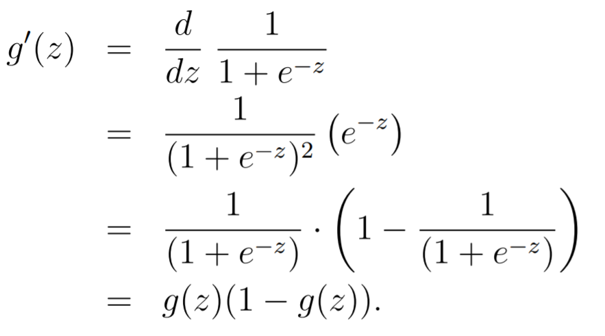
The $g$ is a sigmoid function, and $g' = g(1-g)$ (very helpful identity)

• Derivation

  

A probabilistic view: deriving the loss function

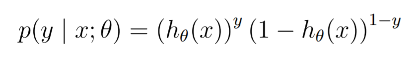
If we look at things probabilistically, we can sort of view $p(y = 1| x)$ as the output of $h_\theta(x)$. It ranges from 0 to 1, and it sort of represents the "confidence" of the model. As such, we can define the following

We can also express this as

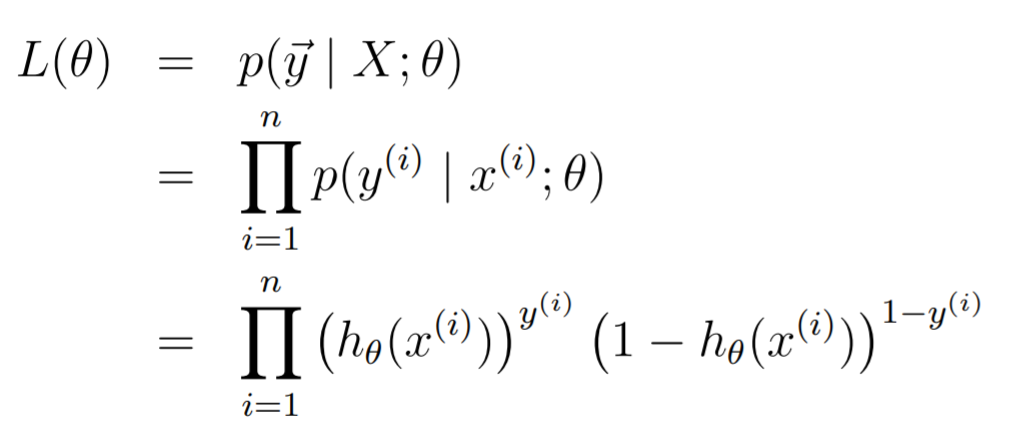
Now, the likelihood is just

And when we do the log likelihood, we get

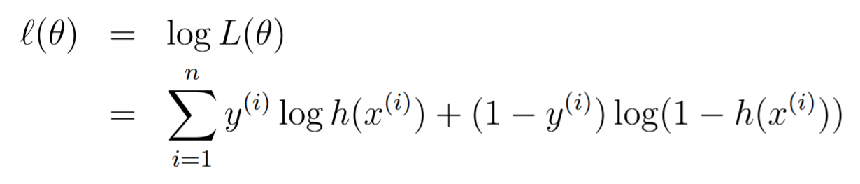
This is our objective—to maximize $\ell$.

Deriving the update

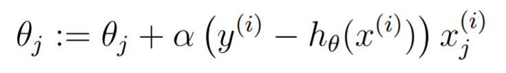
You can take the gradient through this function and you will get the following (using the derivative identity)

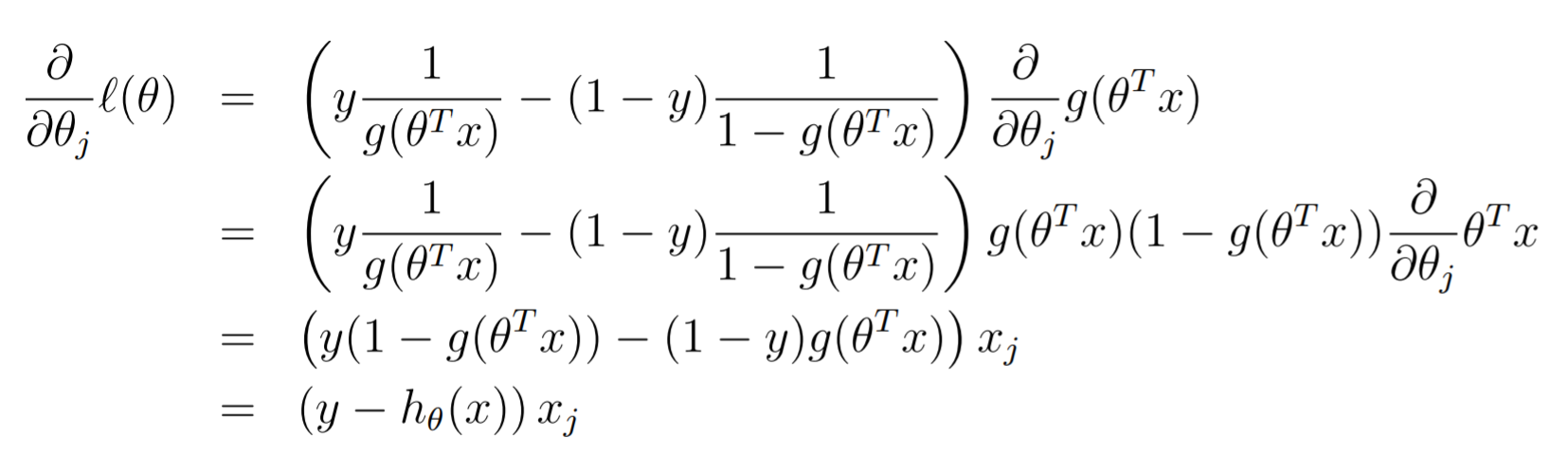
As such, the update is just

If you wanted to find the hessian, it's just

which you can show is positive semidefinite, meaning that it is convex at every point.

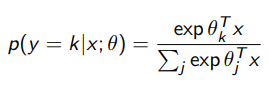
Brief interlude on softmax regression

This is just assuming that the $y | x$ is a multinomial. You can see the math in the GLM section, but you get that

Perceptron learning algorithm

Instead of a sigmoid, if we had a threshold function

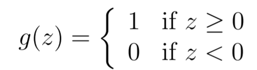
and used the same update rule, we get the perceptron learning algorithm .

The update rule actually has a pretty strong interpretation here. First, let's view the boundary graphically.

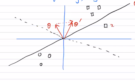
The $\theta$ is orthogonal to the dividing line, because here $\theta^Tx = 0$. Now, say that you got something wrong; you had $y = 1$ but $h = 0$ (shown in the figure). We know that $y - h > 0$, which means that we move $\theta$ more towards the rogue point. However, in doing so, they move the dividing line (dotted line) to include that rogue point.

Partially observed positives

This is a pretty neat problem: what if we had partial observability in a classification problem? Say that we had this setup, where $t$ is the true value and $y$ is the observation

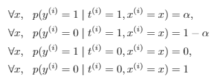
We can show that

In other words, if we observe a positive, then it must be positive.

We can also show that

In other words, the probability of a true positive is proportional to the probability of an observed positive. Taken together, this means that if we wanted to do logistic regression (i.e. model $p(y=1|x)$, the true decision boundary is just shifted a little bit.

To derive $\alpha$, you make the key assumption that $p(t = 1|x) \in \{0, 1\}$. In other words, there is no doubt about the true values. However, you can't assume the same thing for $p(y = 1 |x)$, because it could be a true positive and yet not get measured as one. The probability a true positive is $\alpha$,