The model

• $h$ is the computer, and it's defined as

IF we let $x_0 = 1$, then you can actually create a vector $x = [x_0, x_1, ... x_n]$, which means that

• we call $x_0$ the intercept term.

• We denote the ith element of a vector as $x_i$, and we denote the ith vector in a dataset as $x^{(i)}$. Beware of the subtle difference

The cost function

The cost function is the vertical distance between the predicted value and the real value. We use vertical distance because we care about the line fitting better to the vertical (predicted values) and less so the horizontal values; otherwise we'd use orthogonal distance.

We define the cost function as follows:

Gradient descent

Now, we will update the parameters $\theta$ by this algorithm

Here, $\alpha$ is the learning rate. But what is the partial derivative?

Now, we can use the chain rule and the linearity of differentiation to get the following:

Now, recall that $h_\theta(x) = \theta^Tx$. We know that the partial derivative WRT $\theta_i$ of $\theta^Tx = x_i$. As such, we get

this is known as the LMS update rule (least mean squares), or the Widrow-Hoff learning rule. The summation is for batch gradient descent. You can also use stochastic and minibatch

Normal equations

In this case, we wish to show that it is possible to just solve the optimization problem in one go, without resorting to an iterative approach.

Design matrix

Define a design matrix $X$ to be a $n \times d + 1$ matrix. This means that it has $n$ rows for $n$ training points (batch size) and $d + 1$ features (the one extra features is due to the $x_0$.

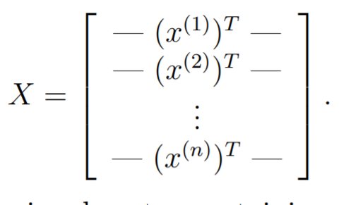
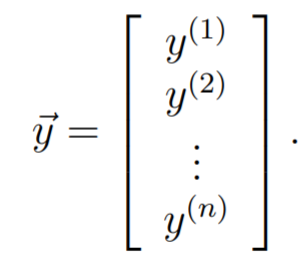
Let $y$ be the vector containing all the target values

The prediction is thus given by

Solving for closed form

As such, the error is just given by

We can derive the gradient through matrix calculus.

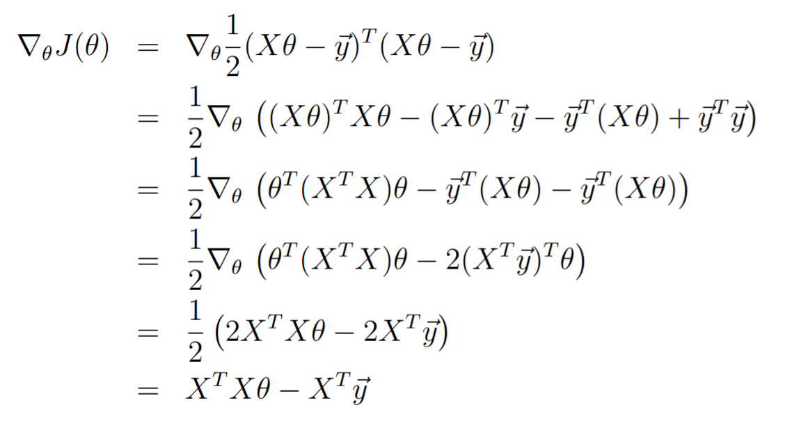
This should be pretty straightforward. The only tricky part is understanding the following forms

• $x^TAx$

• $b^Tx$

And that the inner product is symmetric

this means that the optimal parameter is given by

Connection to Newton's method

This is just newton's method

when the gradient is evaluated at $\theta = 0$. This is why:

So if we started when $\theta = 0$, then newton's method takes one step to converge!

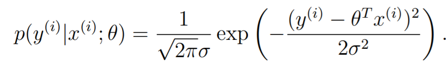
Probabilistic Interpretation

Let's try to understand this one other way: through probabilisty. Let $y = \theta^Tx + \epsilon$, where $\epsilon$ is sampled from an IID gaussian distribution. In other words,

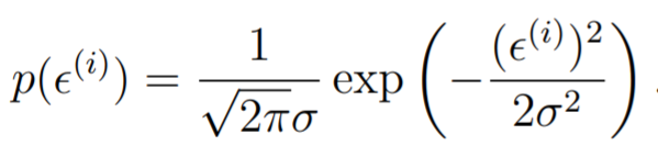
And because $\epsilon = y - \theta^Tx$, we get

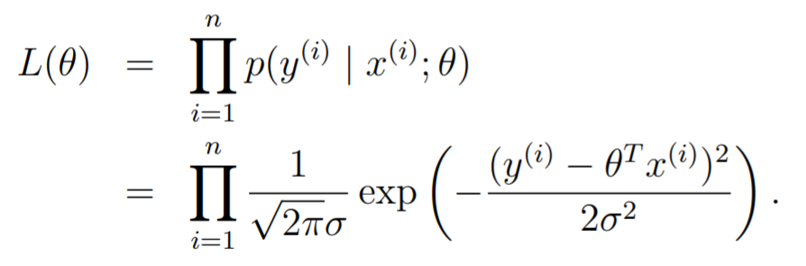
Now, we can understand this to be the likelihood of $y$ occuring given that $x$ happens. When we consider the whole dataset, we get

We will actually maximize the log likelihood, because it allows us to remove the product

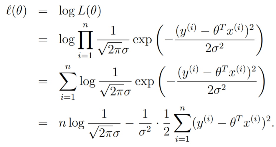
To maximize this log likelihood, we note that we should make the second term that is being subtracted as small as possible. To do so, we minimize

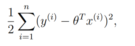
which is EXACTLY what we are looking for!

Generalizing this

This $\epsilon$ doesn't need to be distributed like a Gaussian. It can be any distribution that has some density function $f(z)$. Then, you just plug in $f(y - \theta^Tx)$ into the density function. Calculate the log likelihood as usual, and this becomes your objective (as a function of $\theta$)

Locally Weighted Linear Regression

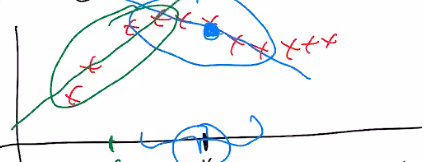
The idea is pretty simple: make the gradients of each point contribute differently. In particular, if you want to predict point $x$, you want the model to fit the points around that point better than the others. Our objective becomes $\sum w^{(i)} (y^{(i)} - \theta^Tx^{(i)})^2$. We typically define the weights as

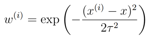
This can be generalized into a vector-valued function as well. The $\tau$ is the bandwith parameter. The smaller the $\tau$, the tighter the distribution and the narrower the window will be. This can result in overfitting. The larger the $\tau$, the looser the distribution and the wider the window will be. This cna result in underfitting.

At run-time, you will take the $x$ you want to predict and run the regression ad-hoc, and then make a prediction. Because we need to retrain the model for every prediction, this is a non-parameteric algorithm. In other words, you can't pre-bake the algorithm and let it run.

The intuition

Suppose that you had something like this. The shape is clearly well-defined, but it might be very difficult to find a good model that works.

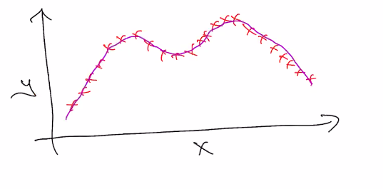
Rather, it might be easier to locally approximate linearity at the points that you want to predict

And from here, you can get pretty good predictions!

Polynomial regression

Polynomial regression is just linear regression in a trench coat. In other words, we can define a feature map $\phi(x)$ that takes in $x$ and outputs $[1, x, x^2, ... x^k]$. In other words, you are taking one point and expanding it into a higher dimensional space. To fit $\theta$, you are still doing linear regression in $\theta$, but you end up with a polynomial regression. Neat!! (which means that polynomial regression is also provably convex)

The objective becomes

This goes beyond polynomial regression; you can use any feature map $\phi$. Because the feature map doesn't get differentiated, the same optimizer can be used.

Parametric vs non-parameteric models

A parametric model is a model that allows you to extract some parameter $\theta$ from the training set, from which you can use for predictions. You can discard the training set after $\theta$.

A non-parametric model is a model that perhaps requires some parameter but also requires the training set to make predictions. A good example is anything with a kernel method.