The simple linear classifier (SVM)

Let’s say we wanted to create a function $f$ that maps from a flattened image into a class vector. We could just use a simple linear classifier

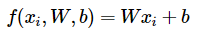
Where $W$ is a $k \times d$ matrix, where $d$ is the size of the image and $k$ is the number of classes. You can actually merge the $b$ into the $W$ if you add a $1$ to the $x$.

To train, we need to make sure to zero-center our data (more on this later) and make the pixels range from -1 to 1

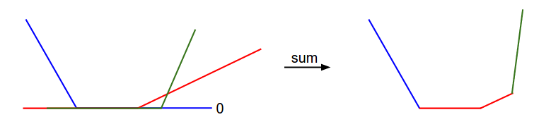
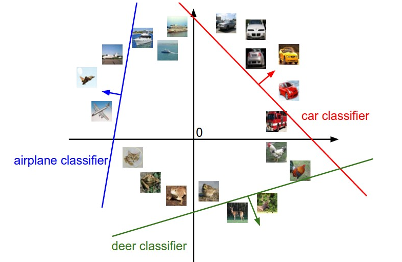
This matrix multiplication you can think of as running $k$ separate dot product linear classifiers. As such, we can visualize this classification as dicing up the hyperspace by a bunch of hyperplanes (the lines represent the zero point in the classifier)

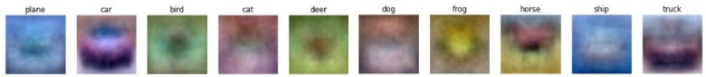
Another interpretation is that each of the rows in $W$ is the “template” image. You are taking the dot product between each of the templates and the test image, and this is just cosine similarity. Here’s an example of what this might look like

Multiclass support vector machine loss

Now, we look at how we might optimize for $W$.

Let $s$ be the score vector: $s = Wx + b$. We compute the SVM loss by running

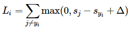
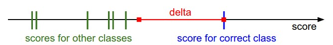
Let’s unpack this for a second. So $s_j - s_{y_i}$ is the distance between class $j$ and the true class $y_i$. Ideally, you want $s_j$ to be very small (negative) and $s_{y_i}$ to be very large (positive). This means that the difference is negative, meaning the whole thing becomes $0$. The $\Delta$ is the margin , which is basically how much breathing room you give. It is a positive number, and it forces $s_j$ to be some $\Delta$ smaller than $s_{y_i}$. Here’s a good visualization

The $\max(0, \cdot)$ is known as the hinge loss

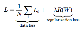
We might add on a regularization term, which acts like Occamm’s razor: we select the simplest $W$ that yields a low loss. It’s mathematically equivalent to a bayesisan prior (see 228 notes) and it helps with overfitting.

Interestingly, this $\Delta$ can be just set at $1$ all the time and we only modify the $\lambda$. this is because the $\Delta$ is just the margin of prediction, and we can change this easily by changing the magnitude of $W$, which of course is modulated by $\lambda$. Therefore, $\Delta$ and $\lambda$ are actually modulating the same thing, and you only need to change one.

Gradient of the SVM

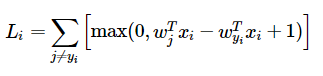
this is something that you are very familiar with from 229 and 228. Just take the gradient! This gives you a closed form expression. For example, for the following SVM loss

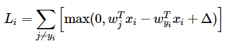
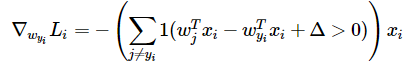
the gradient WRT the target class is

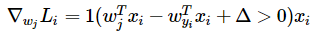
and the gradient WRT all other classes is just

Our eventual goal was to take the derivative of $W$, and we did this by splitting it up into different rows, because that was the most convenient.

Softmax classifier loss function

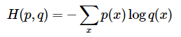
Next, we look at a different, more probabilistic loss function. Why don’t we turn the output of $f$ into a probability distribution, and then take the cross entropy?

Because $p(x)$ is a delta distribution (i.e. a one-hot vector of the true class), we can rewrite this in a simpler form. Essentially, it’s just the softmax term of the true key

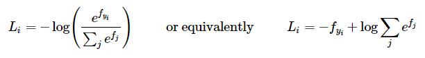
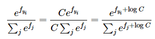
which is equivalent to $-\log p(y_i | x_i; W)$. Just think about it for a second! You want to maximize the log prob by minimizing its negative. For numeric stability, we use a little trick to prevent overflow:

Gradient of Softmax

For target value $k = y_i$, the gradient is

And if $k \neq y_i$, then we have

SVM or Softmax?

SVM is an asymmetric loss. If you’re correct, it doesn’t really care about how much, as long as you beat the margin. Softmax is a smoother loss, and it cares about how much you are correct, as well as if you are correct. This has both pros and cons. You pay less attention to the irrelevant details for SVM. essentially

Topography of the SVM loss

Recall that the SVM loss looks like this

Each $L_i$ is a linear piecewise function, so the final loss function will also be piecewise linear