Feature maps

We talked a little bit about this before: we can reframe polynomial regression as a linear regression problem by defining a feature map

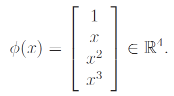
A cubic function over $x$ is a linear function over $\phi(x)$. We call the original input the attributes and we call the outputs of $\phi$ as features. We call $\phi$ thusly a feature map

As we have derived before, linear regression does not depend on what the feature map is. We can just replace all instances of $x$ with $\phi(x)$.

Problem with feature maps

Feature maps go from $R^d → R^p$, and $p > d$. As such, $\theta \in R^p$. The more expressive you want to be, the larger $p$ has to become. This may eventually become computationally intractable. Can we produce some sort of $\theta$ update and prediction algorithm whose complexity doesn't depend on $d$??

The Kernel Trick

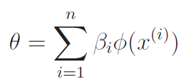
The problem is that the $\theta$ has the same number of elements as $\phi(x)$, which can be very large. The observeation is that at any time, if we start with $\theta = 0$, we can express $\theta$ as a collection of feature vectors $\phi(x^{(1)}, \phi(x^{(2)}), ...$. Now, more formally:

Proving this: induction

The base case is obvious: if we start with $\theta = 0$, then $\beta_i = 0$.

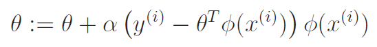
Now, the induction. First, assume that we have $\theta = \sum \beta_i \phi(x^{(i)})$. Now, let's apply the gradient update!

Do you see how we merged into a new expression of $\beta_i$?? That's the trick!!

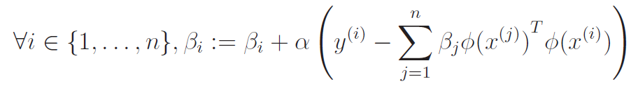
As such, we derive the $\beta$ rule to be (we use ^i as shorthand for ^(i) )

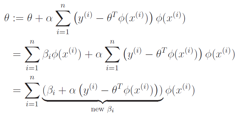
Now, we can expand the old $\theta$ to get

Using the kernel trick: prediction

So we arrive at an important conclusion. We can express $\theta$ in terms of $\beta$ only, and we perform updates using the equation above.

To predict, we note that we want $\theta^Tx$, which we can rewrite using our summation definition of $\theta$. Eventually, we get

Looking at complexity, a prediction is $O(nd)$, where $d$ is the dimension of the feature. We can potentially get past this $d$ if we use a different kernel (more on this in a second)

Using the kernel trick: updates

We have already arrived at the update formulation. Instead of updating $\theta$, we train by updating $\beta$ which by proxy updates $\theta$. We can rewrite the equation above as the update formula simply by replacing the $\phi^T\phi$ with the inner product

Looking at complexity, one update of $\beta$ takes $O(n)$, which means that one whole iteration is $O(n^2)$.

Introducing the kernel

What you might have noticed is that we were able to reduce both the prediction and the update to some sort of inner product. We give this a special name!

The kernel is the inner product $\langle \phi(x^j), \phi(x^j)\rangle$. We formerly define it as

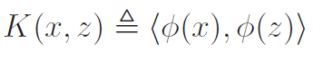
Any function $K$ that can be expressed like this form is a kernel. We will talk more about this in a second.

The power of kernels

We might ask, why does this kernel definition help us? Well, let's look at a concrete example.

Suppose that we had a cubic feature map whose entries were $[1, x_i, ... x_i x_j, ... x_i x_j x_k]$. If $x$ were $d$ dimensional, $\phi(x)$ would have dimension $1 + d + d^2 + d^3$, which is pretty large. But let's actually calculate $\langle \phi(x), \phi(z)\rangle$.

Now, by using summation properties, we get that

Which means that

We have decoupled the inner product computation from the feature mapping!

Kernel functions

There are many kernel functions out there. Above, we looked at the kernel for

In general, the kernel $K(x, z) = (x^Tz + c)^k$ is the polynomial kernel. The corresponding feature map contains the individual parts to the expansion of the polynomial. A polynomial kernel of degree $k$ corresponds to a feature map of dimension $d^k$, where $d$ is the dimension of the input $x$.

For continuous kernels, the most popular one is the gaussian kernel, which is also known as the radial basis function.

We can actually show that this gaussian kernel corresponds to a feature map of infinite dimension.

• Proof

  

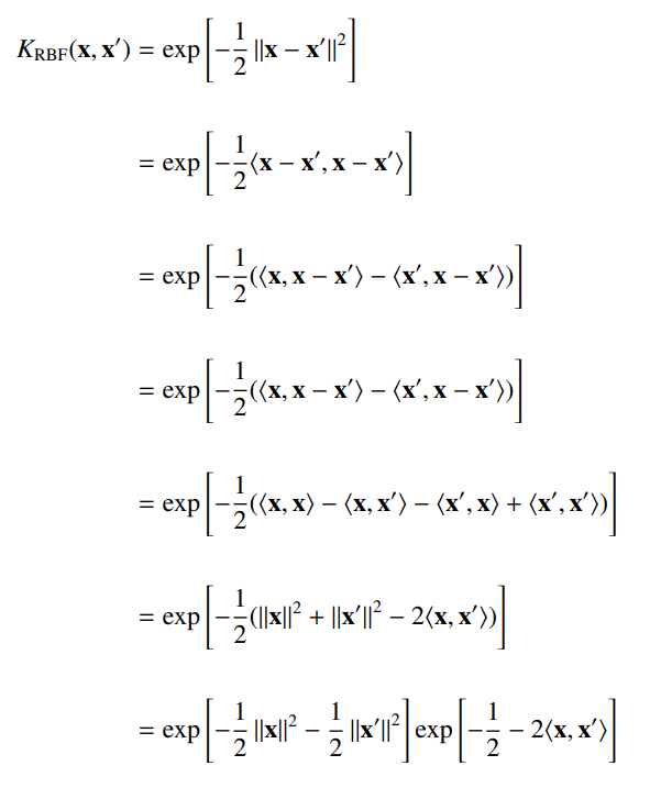
  And then you notice that this is just

  

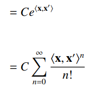
  by the taylor expansion. As such, the RBF is an infinite sum of polynomial kernels. Recall that each polynomial kernel corresponds to a feature map of degree $d^k$, and they all add up. As such, the feature map easily has dimension $\infty$.

There are still other kernels for specialized applications. For example, in a sequence classification problem, we might use $\phi(x)$ to count every possible sequence of length 4 that occurs in $x$.

Picking your kernel function

At the heart, we must remember that the kernel function is some measure of similarity. In sequences, it might be subsequences. In classification, it might be distance. Distance itself is a tricky business.

If you use a simple dot product kernel, the boundary must be linear. Polynomial kernels allow for boundaries of varying curves, and the gaussian kernel allows for circular separation. You can think of the kernel as providing a "separation" factor that is limited to the kernel's behavior itself. Choosing the right kernel is a design choice.

When we make a prediction, we effectively care mostly about the points that are the most "similar", and we look at the $\beta$. Now, these points that are the most "similar" should have $\beta$ with the same sign so that the combined product $\beta K$ will push the prediction one way. Of course, in real life it's more noisy, but with many data points, the majority consensus will win. But this is the intuition of the kernel

Kernel Matrices

We can produce a kernel matrix from the definition of a kernel:

The really neat part is that the kernel matrix can be computed beforehand with a complexity of $O(n^2d)$. This allows training time complexity to be independent of $d$. We can even use tricks like what we described above to compute the kernel without evaluating out $\phi$.

Properties of kernel matrices

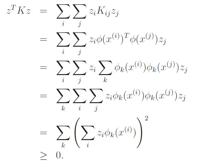
We know that $K$ must be symmetric (property of inner products), and it must also be PSD. We can prove this by computing $z^TKz$ as follows:

• PSD derivation

  

Mercer Theorem

Now, we are going to generalize a bit more. Not only is symmetry and positive semidefinite necessary for a kernel matrix, it is also sufficient. This reverse direction is the work of Mercer's theorem:

If $K: R^d \times R^d → R$, then it is necessary and sufficient if the corresponding kernel matrix is positive semidefinite and symmetric

This means that you no longer need to derive the feature maps to prove that $K$ is a valid kernel; all you need is to prove that it is PSD and symmetric!

• this kinda goes back intuitively to the fact that all $K$ can be defined as an inner product to some feature maps

Proving valid kernels

There's no perfect solution, but if you're dealing with polynomials (like $(1 + x^Ty)^3$), it's best if you kept the transpose notation and started with the summation expansion of $z^TAz$, like

In general, it's good to keep the transpose notation.

In general, here are the things to keep in mind

1. powers of valid kernels (any polynomial) is still valid

2. exponent of valid kernels are also valid by taylor expansion

3. element-wise products of valid kernels are still valid
   • Proof

     

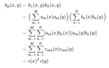
     Essentially you can define a new kernel such that $c_{mn} = a_m * b_n$ and show that this is a dot product

4. sums of valid kernels are still valid (because sums of PSD matrices are still PSD)

Vectorizing with Kernel Matrices

Now, with the kernel matrix, we are able to vectorize the training. The training is as follows: `

(think about this real quick and it should make perfect sense)

Unfortunately, however, the prediction algorithm can't be vectorized because the input $x$ does not have a precomputed kernel.

Kernels above and beyond

Previously, we looked at kernels when it came to linear regression. This is cool, but we can do so much more. How about logistic regression?

Well, we know that the update rule is

Therefore, you can make the same exact kernel trick except you wrap the summation in the sigmoid

You can imagine how we can kernelize other GLM's, and even the perceptron! Pretty neat stuff!