The big idea

In PCA, we tried to formulate a basis that captured the most variation in its axes. In ICA, we also try to formulate a basis, but we try to formulate a basis that "decorrelates" the data.

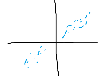
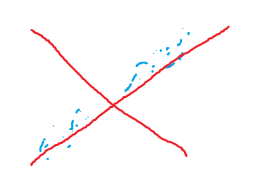
In this example, you see how the left basis creates a correlation in the blue data. But in the right basis, there is no correlation!

We will attempt to motivate ICA again in a more practical case below

The cocktail problem

Suppose that you had multiple people talking at one time, but you wanted to extract the audio from one person. You have multiple microphones so you can get a sense of depth, but how do you parse out this one person?

More formally, you have d-dimensional vector $s$ and you have an observation $x$. The vector $s$ is a random variable that is correlated among its $d$ elements. We want to create a new random variable $x$ whose individual elements are uncorrelated.

A mixing matrix $A$ will "mix" the elements of $s$ and hand it off to $x$, which is also a d-dimensional vector

Can we recover $s$ from $x$? Hypothetically, if $A$ were non-singular, this is totally possible. We can find some $W$ called the unmixing matrix such that $s^{(i)} = Wx^{(i)}$.

So essentially we want to transform as set of random variables into another one

What can't you do?

Well, it's actually more complicated than finding an inverse matrix. The permutation of the original sources are ambiguous, and the scaling is also ambiguous between sources (because you could scale the mixing matrix by $\alpha$ and the source by $1 / \alpha$ and the output would be the same.

In addition, the sources can't be gaussian. Why? Well, we can show that any arbitrary "rigid motion" (orthogonal matrix) applied to the mixing matrix produces the same outcome. First, we can show that $x \sim \mathcal{N}(0, AA^T)$.

Now, we can apply some rigid transformation $R$ such that $A' = AR$. Now, we notice that

Therefore, given a random rigid motion matrix $R$, the output distribution of $x$ will be unchanged!

Densities and linear transformations

If you have a random variable $s$ and you have a transformation $A$, then the density of $x = As$ is not a straightforward as you might think. Imagine if you just put $p(s)$ through $A$. You run the risk of creating an invalid distribution that doesn't sum to 1!

To fix this, let $W = A^{-1}$. A density transformation is defined as

In a way, the $|W|$ keeps tracks of where things stretch and where things squeeze. We mapped $x$ to $s$'s domain by using $W$, but we must account for our stretch debt. This is why the term $|W|$ is there.

For example, le'ts consider the case where $W$ shrinks $x$ twice to $s$. This means that $x$ has double the range, so it should have half the density. Out of the box, the output of the function doesn't change when the input is stretched. This is fine on normal functions, but not on densities that have a clear rule. This is where the $|W|$ comes in, in our previous example—to scale the density by half. Hopefully, this toy example clarifies things.

ICA algorithm

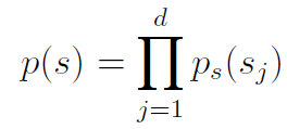
We assume that each source is independent

We apply the transformation $W$ to the data by using the trick we just discussed

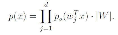
(we just use the row-dot product form of matrix multiplication to convey the different sources $s_j = w_j^Tx)$

The $p_s$ could take any form, and if you knew what the probabilities are like, then you should substitute that distribution. However, in a pinch, we can use the density whose CDF is the sigmoid function $g = \sigma$. As such, $p_s(s) = g'(s)$ and we get

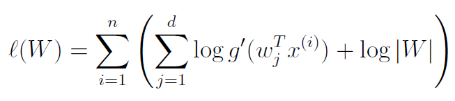
If we take the derivative, we get

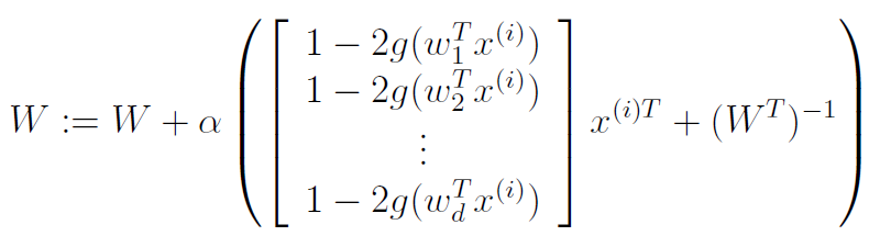
So, after the algorithm converges, all we need to do is compute $s^{(i)} = Wx^{(i)}$.