A new mindset

A probabilistic interpretation of regression is really interesting, because it unifies many things. For example, in our linear regression, we had $y | x \sim \mathcal{N}$, and in our classification one, we had $y | x \sim Ber$. Can we expand to generalized linear models? And what do these even mean??

Distributions, expectations, hypothesis

A hypothesis $h_\theta$ returns a single number given $x$. We know that $y | x$ is a distribution. How does this work? Well, you can think about $h_\theta$ as returning $E[y | x]$. This makes sense in the case of linear regression and logistic regression, and it's a good thing to think about moving forward.

The distribution $y | x$ is a conditional distribution, whose parameters depend on $x$ and $\theta$. For example, of $y | x \sim Ber(\phi)$, this $\phi$ is a function of $x$.

Exponential family

We are about to introduce something a little confusing, but it is needed to work torwards generalized linear models. We define the exponential family as

The $\eta$ is the natural parameter (also known as the canonical parameter), $T(y)$ is the sufficient statistic, which usually is $T(y) = y$. $a(\eta)$ is the log partition function.

The function that gives the distribution's mean as a function of the natural parameter is called the canonical response function. The inverse function is called the canonical link function

When you fix $T, a, b$, you get a family of distributions that is parameterized by $\eta$.

Exponential families include bernoulli, gaussian, multinomial, poisson, gamma, exponential, beta, Dirchlet, etc.

Key properties

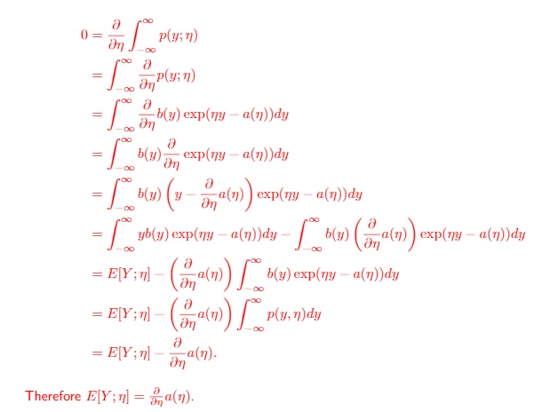
2. $E[y] = \frac{\partial}{\partial \eta} a(\eta)$. This is really neat because it prevents us from integrating.
   • proof: we use a pretty nifty integration trick

     Start from something we know: $\int p(y) dy = 1$. Therefore, $\frac{\partial}{\partial \eta} \int p(y) dy = 0$. However, we can expand this out

     

3. $Var(y) = \frac{\partial^2}{\partial \eta^2} a(\eta)$
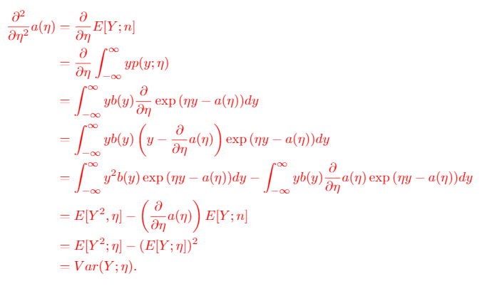
   • Proof: we use what we derived previously

     

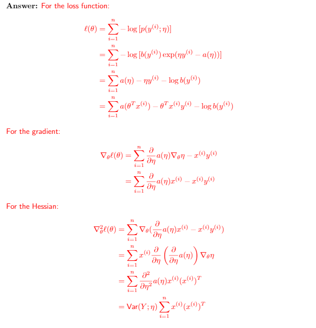
4. when we do a MLE WRT $\eta$, the function is convex
   • proof:

     We will derive the hessian of $-\log p(y)$ and show that it's convex

     

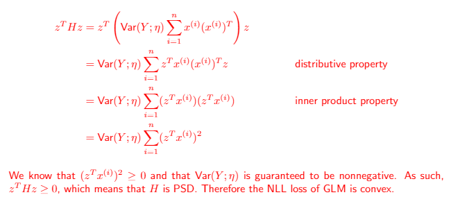
     Now, we just need to show that this is PSD:

     

GLM from the exponential family

To construct a generalized linear model from the exponential family, we make three design choices

First, that $y | x$ is in the exponential family . Second, that the prediction function $h$ is just the expected value of the distribution. Third, that the intermediate parameter $\eta$ is a linear function of $x$ (hence the term LINEAR model)

So the exponential family produces a distribution $p(y; \eta)$. We use this to model what we want, which is $p(y | x; \theta)$. We can imagine the $\eta$ as being a sort of "latent" variable from which the 1d distribution arises.

To get the final model, we derive a canonical response function that maps $\eta$ to the canonical parameters of the distribution like $\phi, \mu$ which give us $h_\theta$ implicitly.

To derive this response function, we just look at $y | x$ and try to squeeze it into the exponential family form.

To summarize:

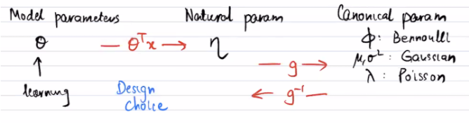
You can actually think of $h_\theta(x) = g(\theta^Tx)$ as an expression of GLM. The $\theta^T x$ is just the $\eta$, and the $g$ is the canonical response funciton!

Optimizing your GLM

The only learnable parameter is $\theta$. Again, think of $\eta$ as your latent variable that $\theta$ helps map to.

For any models in the exponential family, we optimize our model by doing

Or in other words, fit the $y$ with the $x$ with as high of a probability as possible. To derive the update rule, we start with the distribution, like the gaussian for linear regression or the bernoulli for logistic regression. Then, we substute in $h_\theta(x)$ for the parameters like $\mu$ or $\phi$. This substitution turns the original distribution, which depends only on $y$ and some parameters, into a distribution conditioned on both $\theta$ and $x$. This allows you to take the derivative and optimize.

Deriving the general update rule

Our distribution is

By our design, we have

Our objective is to perform MLE, so we can just do log-probability:

Taking the gradient gets us

Therefore, the update is

Interestingly, as we observe, we get $a' = h_\theta = E[y|x]$, which is what we showed before as well.

Derivations of distributions

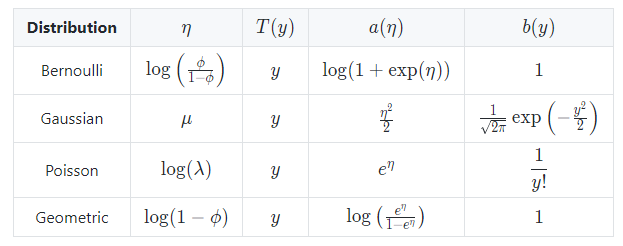
Strategies

1. rewrite things as $\exp \log$. This often loosens things up with inner exponents, etc

2. group all terms with $y$ together. The coefficient becomes your $\eta$

3. Find the canonical response function by solving for the parameter that forms $\eta$

4. Make modifications to the response function to solve for the expectation
   1. for example, in a Bernoulli distribution, you can get $p = e^\eta / (1 + e^\eta)$, but you need to scale it by $N$ to get $E[y | x]$ (which is $np$)

5. Replace $\eta = \theta^Tx$

Let's look at some examples!

Bernoulli as Exponential Family

Canonical parameter: $\phi$

The Bernoulli is in the exponential family. We can expand the equation like this

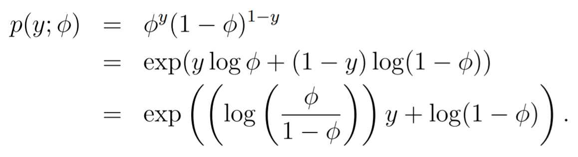
Canonical response function: We see that $\eta = \log \frac{\phi}{1 - \phi}$, which means that $\phi = g(\eta) = \frac{1}{1 + e^{-\eta}}$.

Connection to the Sigmoid

One thing you might have noticed is that the canonical response function is just the sigmoid! This means that if you assume that things are distributed as bernoulis, the distribution's parameters are best described by a sigmoid! Neat!!

Gaussian as Exponential family

Canonical parameter: $\mu$

You can do a similar expanding from the gaussian equation (for now, we assume that $\sigma = 1$

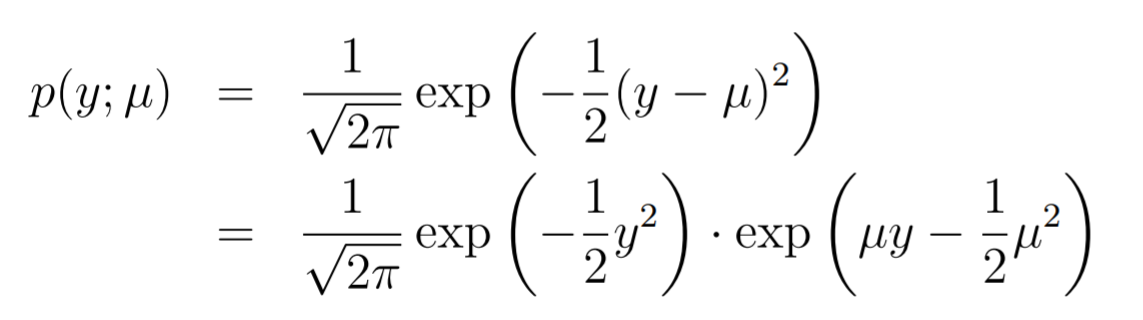
Now, we see that

Here, we see that the canonical response function is just $\mu = g(\eta) = \eta$.

Multinomial as an exponential family

Canonical parameters: $\phi_1, ... \phi_k$, where each $\phi_i$ represents the probability of one outcome. Note how you would need a vector to represent this.

*Because we are dealing with essentially a vector of outcomes, we are dealing with vectors instead of scalars. We have $y$ equal to the "category" of the outcomes, and we define $T(y)$ as

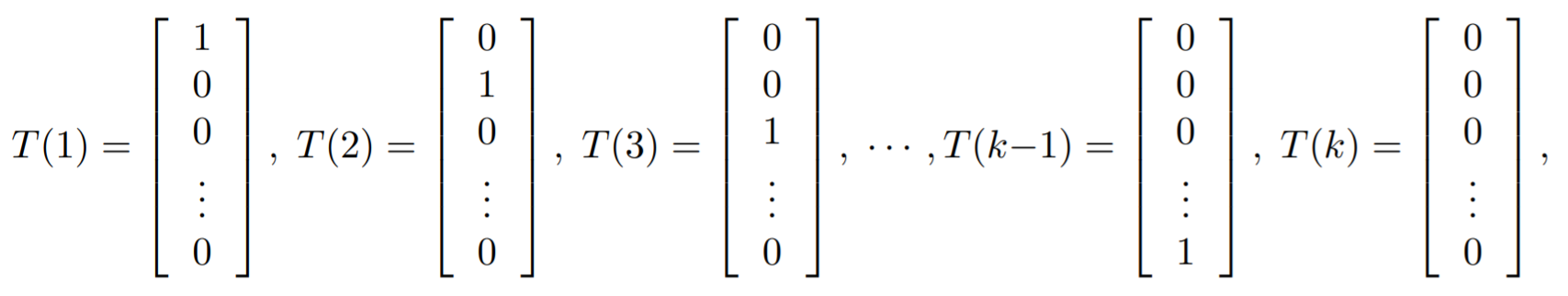
You can also write this as

which will be more important below.

Now, we are ready to derive the exponential family. We start with the multinomial and make our substitutions. It's important to express $\phi_k$ as a sum of other $\phi$, as it is a constraint

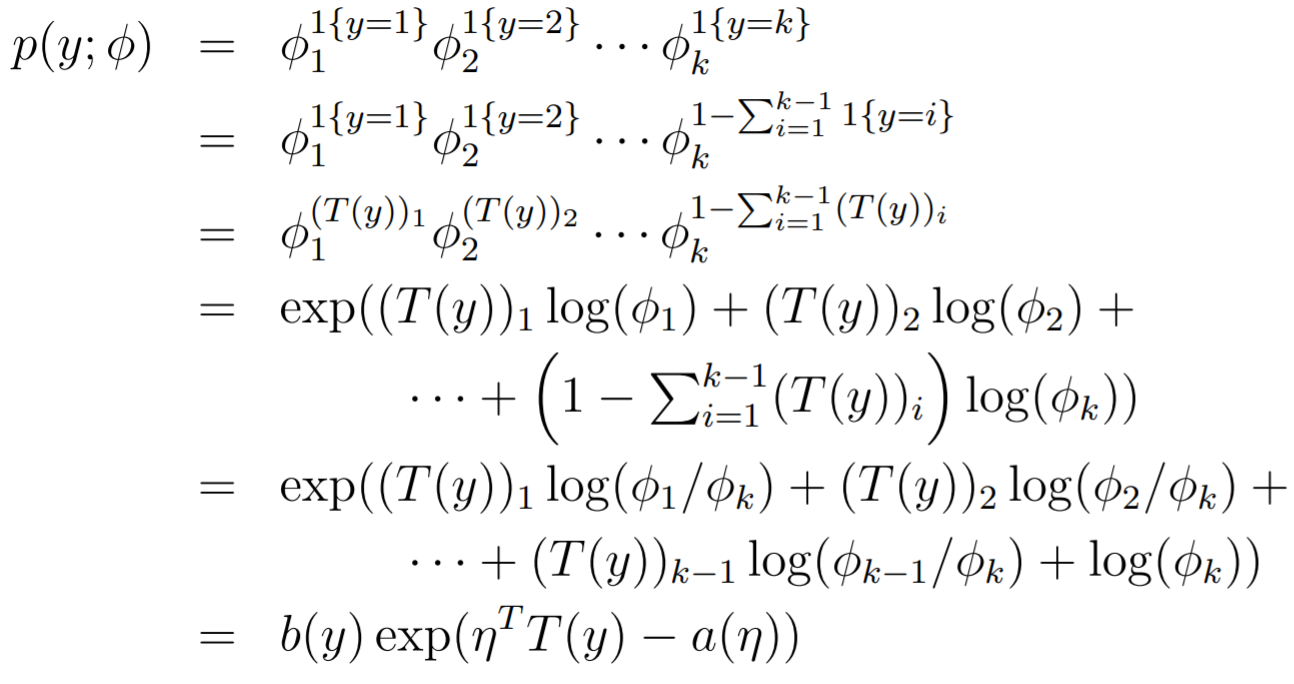
Where

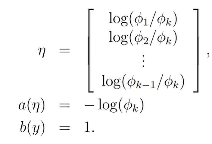
Now, let's look at the canonical response function. If you look at $\eta$, we see that the function is just

To get $\phi_k$, let's use the identity that $\sum \phi_i = 1$:

And this means that $\phi_k = 1/\sum e^{\eta_i}$, which means that

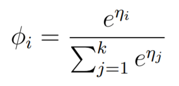
. To recap, what is shown above is the canonical response function for the multinomial distribution, which maps between a vector of logit values to a probability distribution. This is known as the softmax function.

Constructing GLM's

Ordinary Least squares

Recall that $y | x \sim \mathcal{N}(\mu, \sigma^2)$. As such, we have $h_\theta(x) = E[y | x; \theta]$

However, we know that the expectation of a normal is just $\mu$, and we have previously derived that $\mu = \eta$. Therefore, $h_\theta(x) = \theta^Tx$. Neat!! This is what we expected!!

Logistic regression

Here, we actually derive why we use the sigmoid!!

Recall that $y | x \sim Ber(\phi)$, where $\phi$ is defined implicitly with $x$. Now, the following is true:

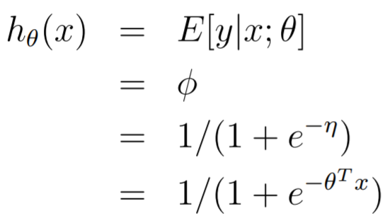
And we arrive upon our logistic regression equation! And this kinda derives the sigmoid function!!

Softmax regression

This one is interesting. Instead of a binary classifier, we have a $k$ value classifier, and we assume that it's distributed according to a multinomial distribution whose parameters $\phi_i$ depend on the input $x$. Now, we have previously derived the canonical response function for the multinomial:

Furthermore, we know that $\eta_i = \theta_i^T x$, so we get the following:

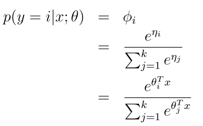
Another way of thinking about this is that we find the logit (the $\theta_i^Tx$) and then we apply a softmax.

Softmax regression: The graphical intuition

The matrix for $\theta^T$ is just a row matrix with one parameter for each class, essentially.

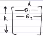
So you can imagine $\theta^T x$ as running $k$ separate linear "tests" on the current point, like the graphic shown below:

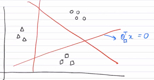
Each of these results are fed into a softmax and we get a probability distribution. The intuition is that the groups are separated by these lines, and depending on how close they are to the boundary, we get different "activations".

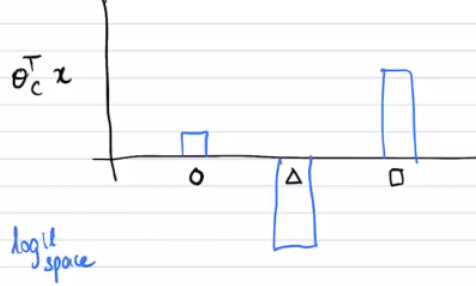
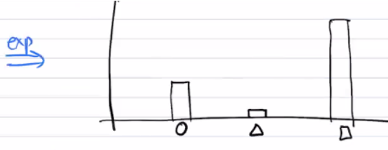
The raw logit results can have a variety of different results, but the one that has the highest score (i.e. the "test" the returns the most positive result of this point being in that class) will have the highest value in the probability distribution.

The tl;dr: softmax regression means running multiple agents and having them vote for which category this unknown point is in.

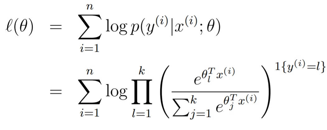
Softmax regression: Learning

To learn the parameters $\theta$, we can use a simple log likelihood:

If you wanted to derive the gradient, it is feasible.

We can also learn using a different, loss-based approach called cross entropy. In cross entropy, we compare two distributions and penalize based on their differences. This is done with the following equation

This is like entropy but it's a mutual sort of entropy. Sampling from the truth $p$, how "surprised" are we to see $\hat{p}$ in a location?