The objective

Given a bunch of points, can I model it while being honest about uncertainty? (i.e. regression with uncertainty)

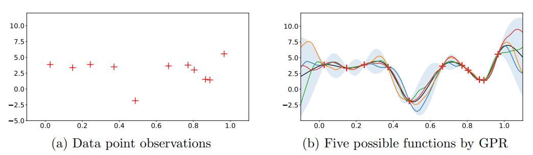
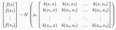
You may choose to sample along the distribution to make your inferences

The approach

Gaussian processes are inherently a bayesian view on regression. You start with a prior on what the function should look like, and then using the points, you compute a posterior on that distribution. But what does this look like?

Modeling the points (the prior)

We assume that the points are sampled from a multivariate distribution. The points $x_1, …, x_n$ is your data, and the $x$ is your query.

You eventually want to compute $p(f(x) | x_1, …,x_n)$, but to do this, we need to know the joint distribution first. This is your prior.

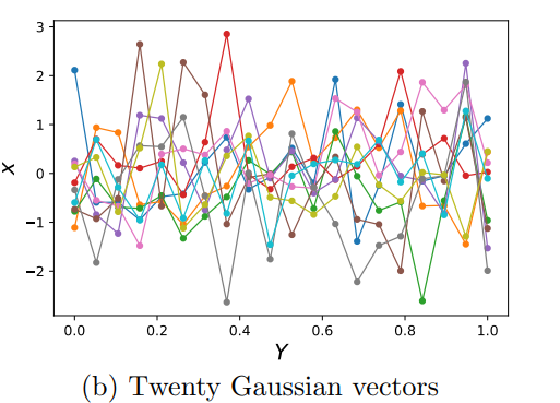
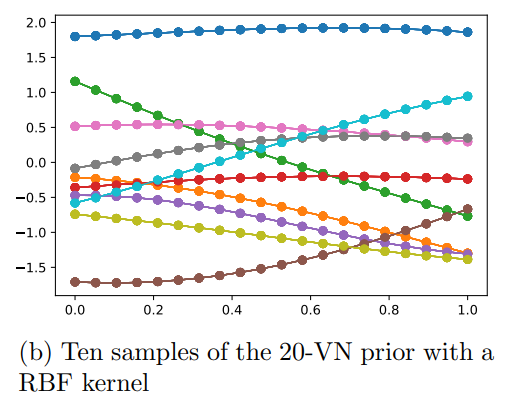
You can express the prior as a bunch of samples in point space. Depending on how strong the kernels are, you get different types of priors

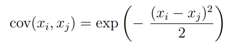
Covariance matrix and Kernel

The covariance matrix above tell us how much correlation some $x_k$ has with $x$. The larger the $k(x_k, x)$, the more the correlation. Usually, we want closer $x_k$ to have closer correlation with $x$. We achieve this through an RBF(radial basis function)

Making the Inference

So we now want to compute this $p(f(x) | x_1,…,x_n)$. How do we do this?

Toy example

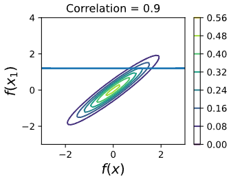
Let’s consider the case that we observe one point $x_1$ and want to compute $f(x) | f(x_1)$. We start with a known two-dimensional distribution $f(x_1), f(x)$.

Well, there’s a visual meaning to this. Conditioning on a gaussian is the same as cutting a line through the graph and looking at the distribution that the line experiences.

The Technical Details

Let’s define the observations as

where $x^k$ is a data point.

Let’s say that we have an input vector $X$ and a query vector $X_*$. The query vector is basically the points you want to predict

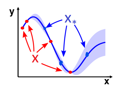
What does this actually mean in terms of our model? Well, let’s say that X is q-dimensional, and X_* is k-dimensional. We want to make an $(k + q)$-variate model that respects our assignments to $X$ and gives a distribution across $X_*$.

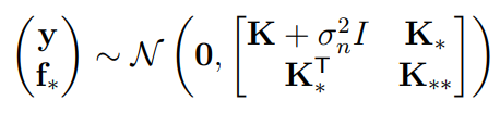
Using the power of block matrix representation, we can actually separate the outputs $f, f_*$ and write them in block form

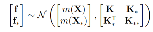
Now, we are ready to condition! We actually know that the conditional of a gaussian is also a gaussian

• Marginal and conditional gaussians facts (also in gaussian section)

  

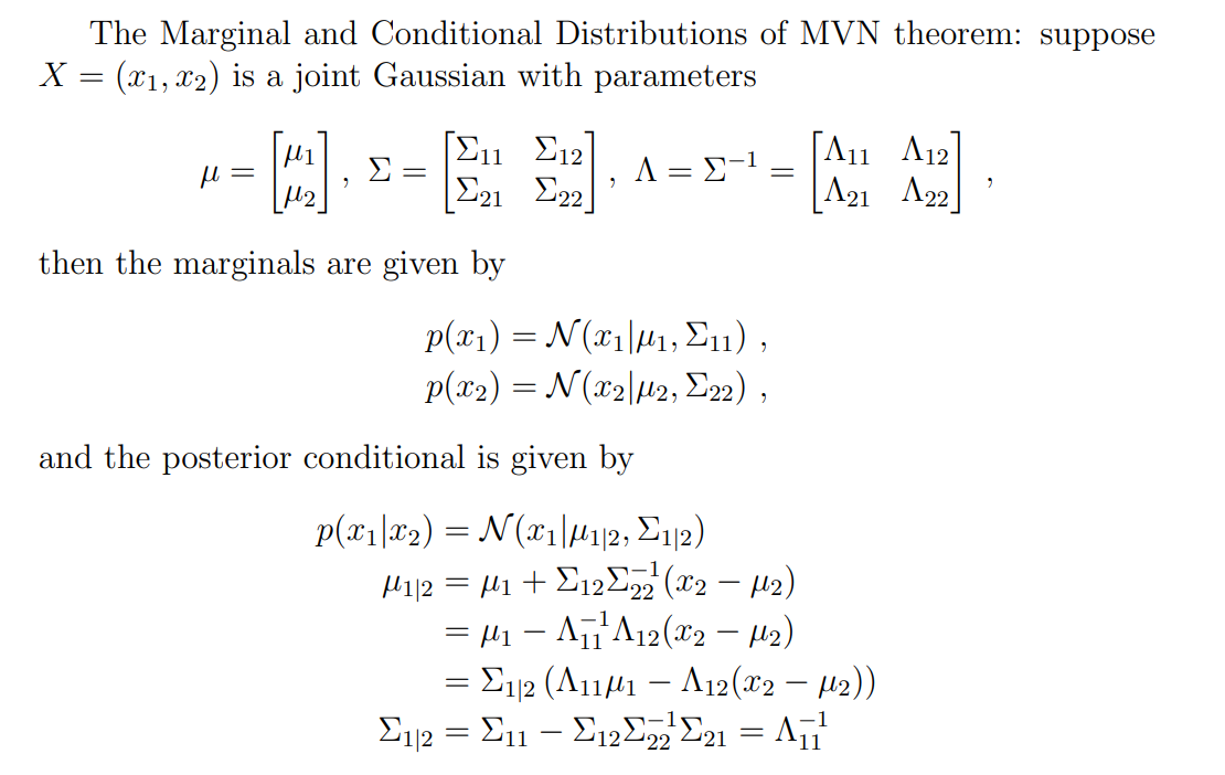
And we know (expand the thing above) that if we get a block matrix representation, we can get the conditional in closed form.

This creates the uncertainty distribution for inference time!

Adding Measurement noise

However, there is always measurement uncertainty, and you can quantify this by adding noise to the original matrix representation. Below, we let $y = f$ symbolically.

And the derivation stays the same (where you see $K$, just add in the noise component)

Moving from one-dimensional regession

In our whole analysis, we only looked at one-dimensional regression. In reality, we can deal with multiple dimensions. Do you see how the kernel function takes in scalars? You can just as imagine a kernel function that maps from vectors to scalars, like an inner product. Then, you would have a matrix of points, with each column representing a data point. The kernel takes care of the rest.