Factor Analysis
| Tags | CS 229Unsupervised |
|---|
The problem
Let be the dimensionality of the data, and let be the number of samples. EM works very well if , so that you have essentially an ability to figure out the gaussian clusters and make insights about it. However, there are cases where , and we are in trouble.
Specifically, these points span only a subspace of the feature domain, so MLE actually yields a singular matrix that can't be inverted for the distribution. The MLE just places all the probability in an affine subspace.
Solution 1: restrictions
Maybe, we can prevent from becoming singular by restricting it into a diagonal. Intuitively, the MLE would be
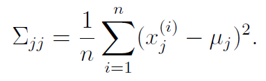
which is just the variance of coordinate . We derive this by looking at our MLE for the non-diagonal () and then just isolating only the diagonal terms.
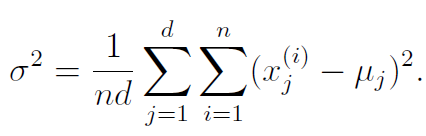
We may also want the variances to be equal, that is, . We can get this parameter by using this formula, which is derived from MLE
From these restrictions, we only need 2 data points to form a non-singular matrix. This is a step in the right direction!
However, we make a strong assumption that the data is independent and all distributed with equal variance. Can we compromise?
Review of gaussians
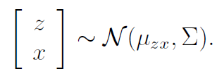
Suppose we had a vector-valued random variable that is consisted of two different vectors
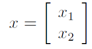
We'd have a mean and a covariance matrix based on this . The covariance matrix is a block matrix
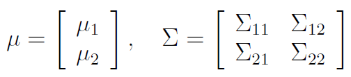
if was length and was length , then would be , would be , and so on. We also know that by symmetry, .
When dealing with block matrices, we have that
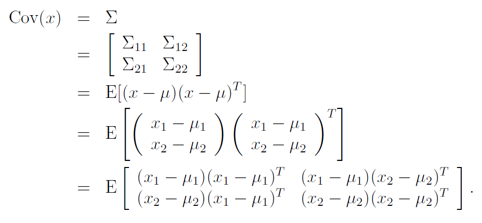
And here's the magic of block matrices! These are almost like numbers and you can treat them as such.
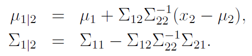
The marginal distribution of is just and the same pattern for . You can show that the conditional distribution is just
Factor Analysis model
Factor Analysis uses a latent random variable such that
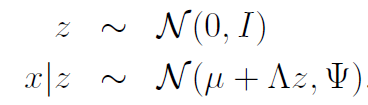
In EM, we assumed that with one mean and variance per , but now we are assuming that there is only one joint distribution but it depends on .
More specifically, is a vector, is a vector, and is a matrix. The is a diagonal matrix. Usually, .
To generate a datapoint, we first sample and then we map it to , and then we add some uncorrelated noise to the outcome. As such, we can also express factor analysis as the following:
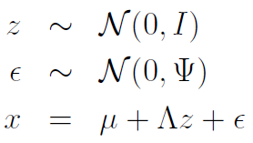
Expressing factor analysis as a joint distribution
Because both and are gaussians, we can think of as sitting in a joint distribution as follows:
The expectation of is always zero, and the expectation of is just
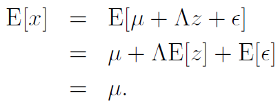
meaning that
What about ? Well, we can calculate and put them together.
First, we start out by observing that .
From the knowledge that and that , we have that
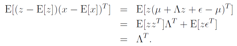
With similar tricks, we also get
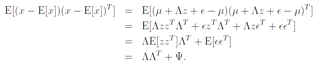
And when we put everything together, we get
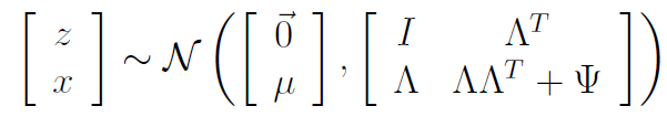
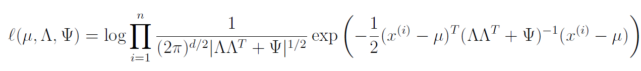
We understand that the marginal distribution is given by
and therefore the log likelihood objective becomes
EM for factor analysis
Maximizing the log likelihood is not very fun, and there's no closed form expression that we know of. As such, we can resort to the EM algorithm.
E step
We can find the conditional distribution for by using the conditional formulas we derived above in addition to the matrix . We will get
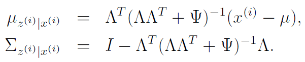
As such, our E step is pretty straightforward

M step,
Our goal is to maximize
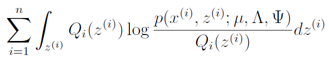
We need to find the optimization for . We start by simplifying the expression using log rules
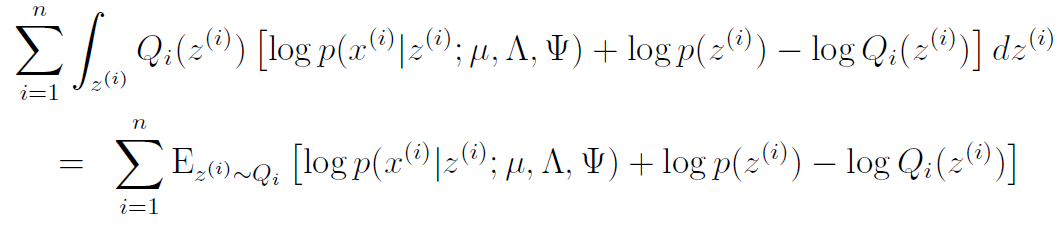
Now, we will focus on as an exercise. We'll tackle the other parameters later. Therefore, we can eliminate certain things that we don't need. In fact, we only need to keep the first term
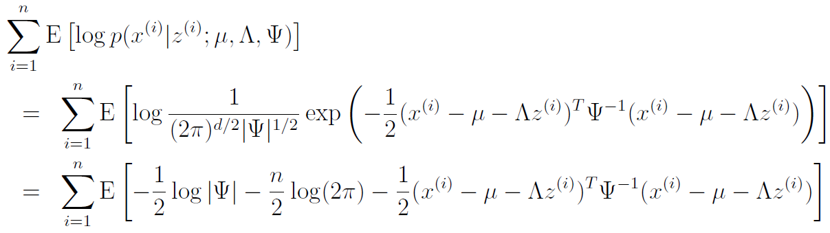
And we keep only the relevant terms again and using some trace properties, we get
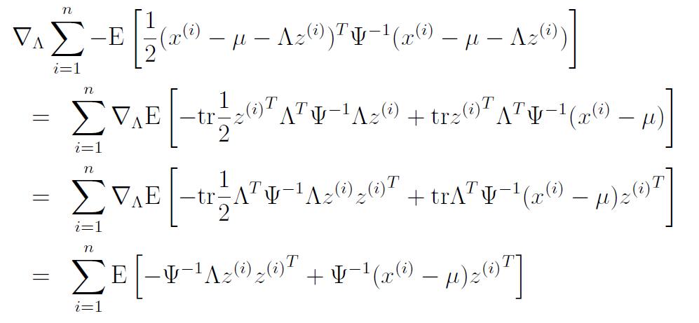
We can set this equal to zero and simplify
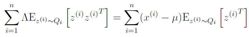
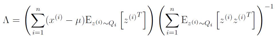
If we use the identity , we get that
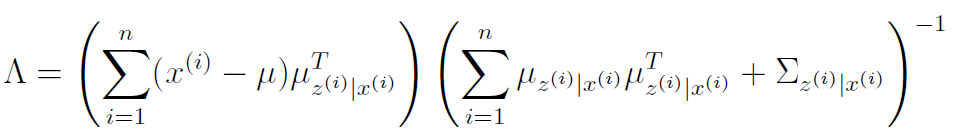
M step,
It can be shown that the M step yields
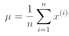
and as for , we calculate as follows:

then, we set .
So what are we doing again?
Our big goal for factor analysis was to represent high dimensional data in a way that we can perform EM algorithm on. We did this by sampling a lower-dimensional vector, projecting it up to the high dimensional space, and adding independent noise.