The big idea

Small trees and small models in general are easy to train. However, they have a high bias. How do we get a stronger classifier?

We could add more features, depth, etc. Or, we COULD boosting.

Boosting is the process of combining primitive networks together into ensemble models.

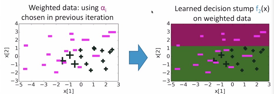
More specifically, we start with some primitive model $f_1$, train it, and then make some updates to the dataset to mark where $f$ did the worst. Then, we train another model $f_2$ (usually of the same type) and repeat.

Boosting, formalized

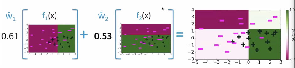
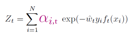
We have a bunch of primitive models $f_1, ... f_n$ that output either a -1 if it predicts one class, or a 1 if predicts the other class. We will define as master model as

Weighing

There are two sets of weights we need to care about. First, we care about the weights of the contributing models: $w_i$. Second, we care about the weights of the evolving dataset: $\alpha_i$. if each model were trained on the same dataset, then we would just have a bunch of the same models! The key insight here is that we let the performance of the previous model CHANGE how we weigh our next dataset.

Weighing: the $\alpha_i$

Each datapoint $x_i, y_i$ is weighted by $\alpha_i$. When training, data point $i$ counts as $\alpha_i$ data points. Intuitively, this marks the "hard" spots for the next model to focus on

• A good diagram

  

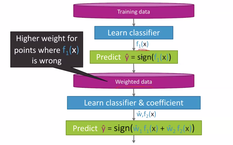
Weighing: the $w_i$.

We will talk more about this, but essentially the $\alpha_i$ is "how importance is this point" and the $w_i$ is "how important is this model's contributions?"

The Adaboost algorithm

The adaboost algorithm is a very slick way of provably optimizing for the different weights. Here's the overview

For t = 1, ...T:

1. learn $f_t$ with data weights $\alpha_i$

2. Compute coefficient $w_t$

3. recompute weights $\alpha_i$ based on how the model performs now

To predict, compute

Computing contribution weights $w$

Let's focus on binary classifiers for the setups below.

There's a very intuitive way of calculating $w_t$. if the model had a higher error, then we should care about it less. We should be considering a weighed error with $\alpha_i$ weights because then we know if our objective is being reached. We can summarize these points up as the following equation:

• as the weighted error approaches zero, the weight approaches infinity

• as the weighted error becomes 0.5 (essentially flipping a coin), the computed weight is 0 (essentially "ignore this")

• as the weighted error becomes more than 0.5, the computed weight becomes negative. This is because errors greater than 0.5 means that your model is good if you flip the labels! (think about this for a second). The negative weights automatically do this

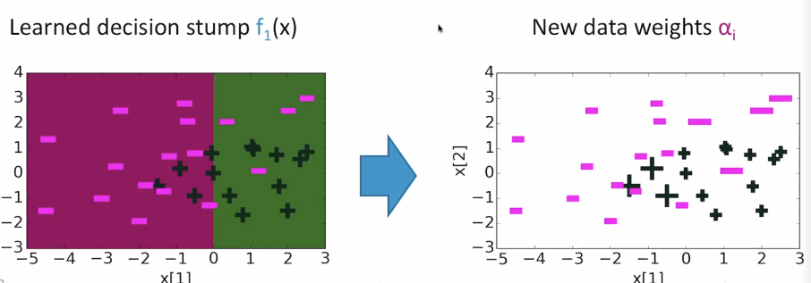
Computing dataset weights $\alpha$

This is also pretty intuitive. If the model predicted correctly, we should decay the importance of that point by its confidence. In contrast, if the model predicted incorrectly, you should boost the importance of that point by its confidence.

Intuitively, if you're right and you're confident that you're right, you don't need to see that point again. However, if you're wrong and you were confident about it, then you really need to see that point again.

So:

• if $f_t(x_i) = y_i$, then $\alpha_i := \alpha_i e^{-w_t}$

• if $f_t(x_i) = y_i$, then $\alpha_i := \alpha_i e^{w_t}$

Normalization

If we make a mistake on $x_i$ often, the $\alpha$ can get very large, and if we are correct, then the $\alpha_i$ can get very small. This can cause numerical instability, so we normalize the weights

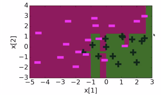
Adaboost, visualized

and after 30 iterations, it looks like this:

Adaboost: optimization theory

There is only one condition: at every $t$, we must find a weak learner with a weighted error of less than 0.5. This is easy, but not always possible. As an extreme example, if your positive examples and negative examples were EXACTLY the same points, you would not be able to achieve this.

Establishing the upper bound

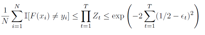
We can show that

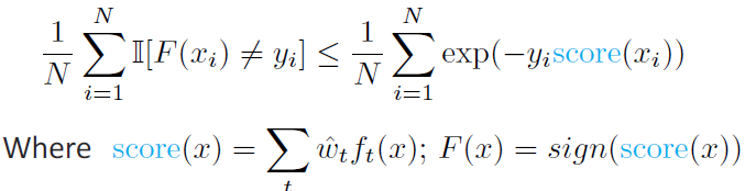
For a hot second, let's forget about the summation. On the left hand side, the loss is 1 if it's not equal. This means that $y_i$ and $score(x_i)$ did not have the same signs. If we plot $y_i * score(x_i)$ vs loss, we'd get a step function as the left hand side (see below).

Now, let's look at the right hand side. That's just an exponential!

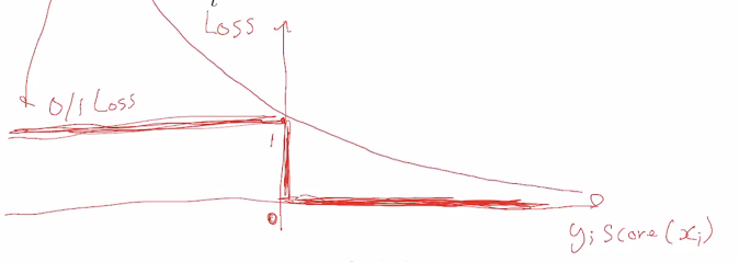
So this is why we have the upper bound on the loss.

We call this a surrogate loss, and it's a neat trick whenever you're dealing with non-differentiable losses: just make a worst case, and show that it converges!

How do we do that??

Convergence guarantees

We can actually rewrite things as follows:

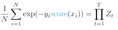
Here, we see a change in summation to product, as well as what we are operating across. $Z_t$ corresponds to a model, not a data point.

Now, as long as $Z_t < 1$, the more models you add (increase $T$), the closer the upper bound on training error gets to zero. As such, as long as you keep this condition, you are guarenteed to converge!

If you minimize $\prod Z_t$, we minimize our training error. We can achieve this greedily by minimizing each individual $Z_t$. If you do the derivation out, you note that

As such, your best bet is to minimize $Z_t$ by changing $w_t$. As it turns out, the optimal solution is

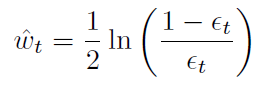
where $\epsilon_t$ is the weighted error of $f_t$. This explains the adaboost weight update step!

In general, we can describe the optimization as above. If each classifier is at least slightly better than random, then we have $\epsilon_t < 0.5$, which means that the exponenti will always be negative and increasingly negative with increasing $T$.

Boosting vs decision trees

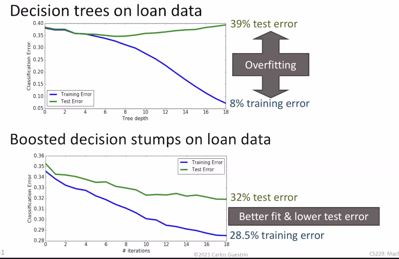
At the heart, boosting is like adding nodes to a decision tree, but you have some control of how each node contributes. The additional degrees of freedom makes the boosting algorithm more robust to overfitting

Ensemble models are useful in computer vision and most deployed ML systems use boosting because they perform so well!

Tuning hyperparameters

• the number of trees you use should be done through a validation set or cross-validation set

Other species

Gradient boosting: like Adaboost but generalized to anything

Random forests: pick random subsets of the data, learn a decision tree for each subset, average predictions. Simpler than boosting and easier to parallelize (doesen't need to depend on the previous predictions). However, it typically has higher error than boosting for the same number of trees