Visualizing CNNs

Weights

Before, we were able to visualize the weights to a linear classifier, because the rows of the matrix corresponded to template images.

We can do the exact same thing to the first layer of the CNNs. We can take each filter (if the next layer has $k$ depth, there are $k$ filters) and display it as a 3-channel image (because the first layer is 3 channel)

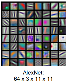
You can also visualize the raw weights on an internal layer, although it often makes not much sense because it doesn’t have a good color interpretation

Embeddings

We can also chop off the head from the network, so that you are left with a high-dimensional embedding. For example, you might take the second to last FC layer as the vector.

Then, you can use this embedding to run K-nearest neighbors, which leads to a much better semantic similarity than just raw pixel space

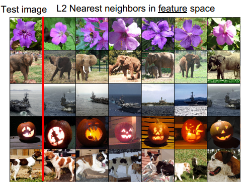
You can also perform dimensionality reduction on the embedding and run things like PCA or t-SNE, which allows you to plot the images on a low-dimensional space (like 3d)

Activations

You can also visualize activations, which help you figure out essentially what each layer is looking for.

Understanding inputs

Maximally activating patches

If you run a bunch of images through a network and recorc the values of some channel in some layer of the network, you will start to see which images activate a channel the most.

Saliency via occlusion

You can also run a sliding window over the image to see which parts of the image are impacted the most. This allows yo uto generate a heat map, essentially, of importance.

Saliency via backprop

The key insight here is that we don’t have to rely on these probe-and-done methods to figure out the importance of something. The computational graph takes us from the image to the prediction, so we can take the target probability and take the derivative of the image with respect to the target probability.

This allows you to segment the image (anything without much importance to the classifier can be removed, or set to 0)

This also allows you to detect biases and shortcuts. Sometimes, the model might learn to pay attention to the background and not the main subject.

Intermediate features through guided backprop

Why stop at figuring out which pixels change the prediction the most? You can also select a single intermediate neuron and figure out which pixels in an image activate it the most.

Gradient ascent

If we are taking gradients, why stop at figuring out the magnitude of the gradient? We can also take a step in the gradient! This would mean you are generating an image of a desired type.

You should also put in a regularizer to make sure you get a resonable image.

if you start with a zero image and run this gradient ascent, you get something like this

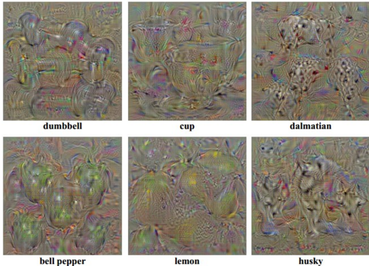
To make things better, you can blur the images (spreading out the gradient) and clip both small pixels and small gradients (to reduce noise).

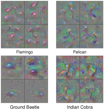
Now, you can also do the same trick with the intermediate neurons to figure out what activate the neurons the most

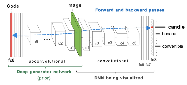
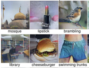
You can also have this upconvolutional step, which allows you to generate much more realistic images

Adversary

With the previous images, we’ve tried to work with the image to make it more likely to be classified to its original category, or we’ve generated things from scratch. We can also move an image and optimize it such that it’s falsely categorized, using the same gradient ascent optimization objective. This is known as a fooling image

You can also find a universal perturbation through gradient descent that messes with as many images as possible

Style transfer

Feature Inversion

If you start with the embedding vector (at the end of the CNN), you can try to find another image that matches this vector as closely as possible, which is just another optimization problem. Depending on where you sample the feature vector, you can get a whole range of generation

DeepDream

The gist here is to take an image and a layer in the network, and then perform gradient ascent on that neuron WRT the image such that we boost every activation in that layer. This is akin to a lucid dream, where there is this hyperreality.

The deeper you select a neuron, the more complex features will show up

Texture synthesis & Gram matrix

The gram matrix is the outer product formed by pairwise slices through the channels

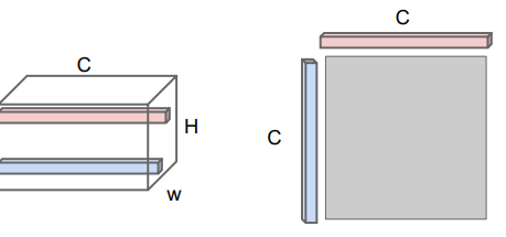
The outer product is the highest if both values are the same, and so it measure co-occurence. This can be easily computed if you flatten the activation into a $C \times HW$ matrix $F$ and do $FF^T$.

Another way of understanding this is a pairwise dot product between channels. The idea here is that we remove spatial considerations and keep the variances between the channels, which can be representative of the styles

It’s just a sloppier and faster version of the covariance matrix, and it is associated with style, because style is a sort of “variance” in the image.

To synthesize texture, you should run the seed image and the target image through the network, and then backpropagate to have the target image and the seed image have as close of a gram matrix as possible. The later the activation used to compute the gram matrix, the larger the transferred features.

Feature + gram

If you have a dual objective of making the features of an image the same as a target image, as well as making the gram matrix the same as a style image’s gram matrix, you are able to transfer the style onto a real image

You can also do a fast style transfer by using a CNN that stylizes it in a feedforward pass. Essentially, you’re learning the backpropagation.

Style transfer helped develop the instance norm, which averaged across pixels but not channels or batches.