What is self-supervision?

Self-supervision is using a bunch of unlabeled data and doing stuff with it to develop a feature embedding that can be useful for later, supervised tasks.

Pretext tasks

You can make some “puzzles” for the model to figure out without needing any labels.

Rotations

Given an image, what’s the rotation? You can have a continuous model, or you can have a 4-vector output prediction. This is productive because to infer rotations, you need to have a semantic understanding of “things” and what they usually look like. The model, RotNet, is able to outperform a collection of other pretraining methods.

Patches

You can predict relative patch locations. given two patches, what is the one patch’s location WRT the other?

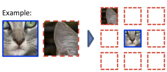
You can also give a bunch of patches and have the model predict how they are re-assembled. Usually, these models output a number which is mapped to a pre-defined permutation. This is a supervised problem because we can make these patches without actual image labels.

Intuitively, this performs well because you need to understand the macro structure of an image in order to reassemble it.

Inpainting

Given a blank part of an image, can we paint something that is convincing?

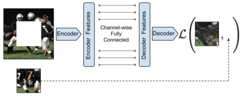
We can use a simple L2 loss added to an adversarial loss. This is because we want our model to seem relevant to the scene (L2) but also have the right “vibe” of the scene (adversarial)

Image coloring

Given a greyscale image, can you output the color version? You do this in the LAB channel space, where L is the greyscale, and you give the AB color information. Here, a split-brain autoencoder can be used, which maps between two domains in separate streams.

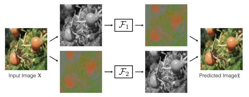
Again, you’re not trying to solve a problem here, so this is why this setup seems a little stupid. But in reality, you’re creating feature embeddings in $F_1, F_2$ which can be helpful down the line.

Video coloring

We can also try to color videos. You have a colored reference frame and then you have a target frame. When you run the CNN you get an embedding $C \times H \times W$. You extract channel cores from the reference and target embeddings and you compute attention maps

Then, the predicted color is just the weighted sum across $A_{ij}$ and the reference color

in total, this looks like this structure

Now, with this model, you can create segmentation masks! If you can figure out how colors flow, it’s simple to replace the colors with a mask. The key here is that there is a sort of learned attention, and this is widely useable.

Contrastive learning

Contrastive representation learning

Basically, if you’re given a base image, positive image, and negative image, you want to push the base and positive image features as close as possible, and the base and negative images as far apart as possible.

InfoNCE loss

We can use the InfoNCE loss, which is defined as the following:

Essentially, you are given 1 positive example and $n-1$ negative examples. Your loss is just the softmax across the raw scores. In other words, you are just training an N-way softmax classifier, where the one-hot vector is the location of the positive example. Mathematically speaking, $-L$ is the lower bound on the mutual information between the base $f(x)$ and the positive example $f(x^+)$. By minimizing the loss, you are making $f(x)$ and $f(x^+)$ be as dependent as possible.

SimCLR

This is a simple idea. You actually don’t have to use negative examples anymore

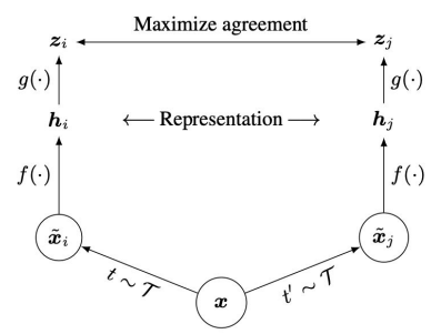
Basically, you train a $f$ that embeds an input, and then a non-linear projection $g$. You want to make these as close as possible. The insight here is that $g$ will force the represntations to capture the relevant big ideas, while allowing more information to be kept in $h$. The agreement of $z$ is measured in cosine similarity.

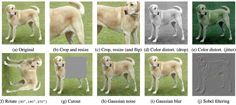
There are many augmentations that you can use:

To vectorize this, you stitch together the features into a matrix, and then perform matrix multiplication. Then, you select the elements that are relevant.

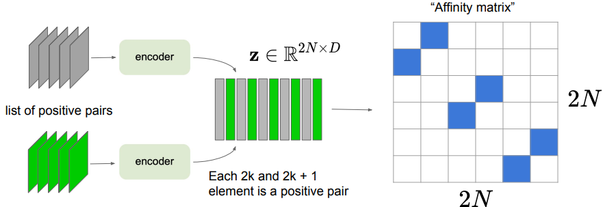
The problem is that it requires a large batch size, probably due to instability.

MoCo (Momentum Contrastive Learning)

You have a query input, as well as a queue of negative samples. You encode the query using a function parameterized by $\theta_q$. You encode the negative examples using a function parameterized by $\theta_k$. These are related through a slow momentum update $\theta_k \leftarrow m \theta_k + (1 - m)\theta_q$.

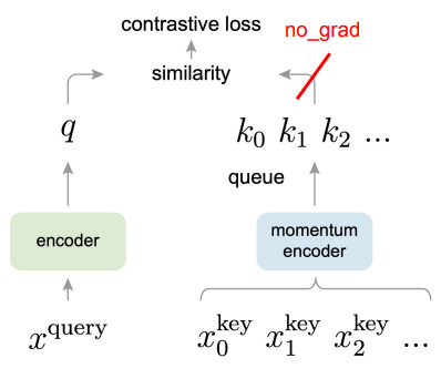
We compute one positive example and $q$ negative examples, then use the InfoNCE loss for optimization. After each step, we update $\theta_k$.

MoCo v2

They took the best of SimCLR and MoCo and put it into one model. They added a non-linear projection head and strong data augmentation from SimCLR. They kept the momentum-updated queues

Contrastive Predictive Coding (CPC)

Basically, you use a positive sequence where a pattern is upheld, and a negative sequence where a pattern is broken

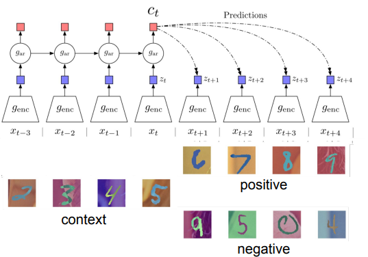
We transform $c_t$ of the state by using a weight matrix $W_k$, where $k$ is the step that the pattern-completer is on.

You might also use this idea to predict images by looking at patches in the image again

Other examples

There is CLIP, which minimizes the encoding distance between speech and music. With pixel-wise features (these exist), you can even map between pictures.