Things to look out for

We worry about memory and parameters. Memory is the amount of space the activations take up. Parameters is the count of the numbers needed to define the network. As a general rule of thumb, the memory is high early on in the network, and the parameters are high when we flatten the final image

Layer Patterns

Now that we know how CNNs are constructed, we can begin looking at some canonical structures.

The most common is something like this

INPUT → [[CONV → RELU] * n → POOL / LARGE STRIDES] * M] → [FC → RELU] * K → FC

General tips

• pooling is distructive, so to make your network more expressive, use a few stacked convolutions per pool

• Prefer stacks of convolutions with small receptive fields to one convolution with a large receptive field. This is because the non-linearities make it more expressive. It is also more efficient in terms of weights.

• If you are using convolutional neural networks for something, use whatever works best on imagenet. Don’t try to reinvent the wheel.

Common hyperparameters

• Input layer should be divisible by 2 many times

• The convolution should use small filters, around 3x3 or 5x5 using stride $S = 1$. Larger filters (like 7x7) should only occur at the beginning, if any

• The inputs should be padded such that each convolution keeps the same size. If we don’t do this, the information at the borders are artificially disregarded (because the filter physically stops before it is able to cover the borders appropiately)

• Pooling typically uses a $2\times 2$ receptive field with a stride $S = 2$, which means that we take tiles of 4 pixels and either take the mean or the maximum.

AlexNet

8 learned layers. There are 5 convolutions and 3 fully connected. They use the ReLU in the CNN, which is a novel approach. They also use normalization and overlapping pooling.

Due to computational resource constraints, they had different GPUs running separate stacks of the convolution. In other words, they split the filter stacks across GPUs.

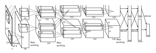
To reduce overfitting, they augment the data. They also use PCA on the colors, which helps with color invariance.

They also used dropout, which essentially randomly samples an architecture by zeroing out a set of neurons at random, which forces a form of neuroplasticity. During test time, they use all the neurons but they scale it down. If they had 60% dropout, then they would multiply each activation by 0.4, etc.

VGG

They used a variety of architectures and they stuck with smaller filter sizes (including 1x1 convolutions). It shows that deeper and bigger networks work better.

The philosophy is that stacks of smaller convolutions have the same receptive field as a larger convolution layer, but at lower computational complexity and higher expressivity (because of the nonlinearity)

As an example, 3 of the 3x3 convolutions have the same field as a 7x7, the 7x7 has $49 / 27$ more parameters (nearly double)

As we go through the network, we halve the H and W through pooling, and we double the depth. This has an overall effect of halving the activation count (think about it!)

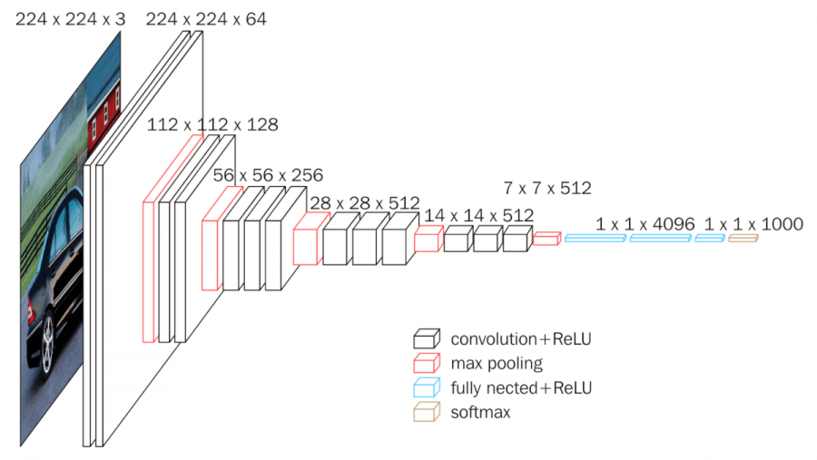
There are a few versions, including VGG16 and VGG19.

GoogLeNet

This model realizes that deeper models can yield higher complexity because you have to propagate things through an entire chain. Instead, these authors decided to widen the network by essentially making a bunch of ensemble models and concatenating them. This allows us to try multiple different filters, which can give us more information.

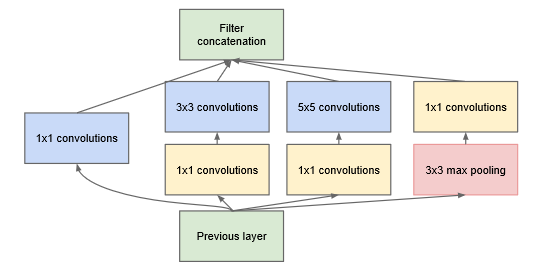
The inception module applies different sets of filters and concatenates them depth-wise. Now, to reduce complexity, there is a bottleneck 1x1 convolution that reduces the depth of the input before running through a convolution. This, again, is equivalent to taking each pixel and running a FC net on it that reduces dimensionality.

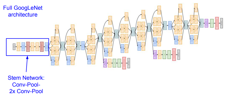
The whole infrastructure consists of many inception modules stacked on top of each other. There are auxilary heads that allow for gradient injection in the middle of the structure, which helps with optimization.

Another trick that the model uses is they do a global average in the final feature map. Perhaps a diagram makes more sense here

ResNet

Previously, deep CNNs aren’t making much progress because the gradient likes to die before it can impact all the parameters.

The authors of this paper ended up rethinking the role of a convolution. What if, instead of creating a whole new activation, the convolution just decided what to modify from the previous activation? And thus, the residual network was born.

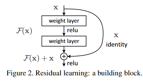
For same-shape activations, this is a straight addition. For non-same shape, they use a projection matrix $W$and add $Wx$ to the activation.

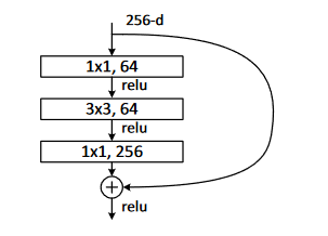
To reduce complexity, they also use a bottleneck layer, which uses a 1x1 convolution to reduce the depth just for the real convolution, but the “backdoor” still operates in full dimensionality.

Other advancements

You can add a feature recalibration module that adaptively reweights each depth slice

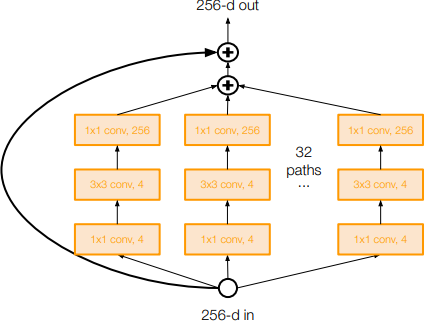
You can make residual networks wider by adding more filters

You can fuse residual and GoogLeNet

You can have densely connected convolutional netural networks, which means that each activation is connected to all the activations in the future